


The Habitable Planet: A Systems Approach to Environmental Science
Atmospheric Pollution Online Textbook
Courtesy United States Environmental Protection Agency.
Geography, climate, and a high concentration of pollution sources create endemic air pollution problems in the Los Angeles basin.
1. Introduction
Unit 11 // Section 1
The first week of December 1952 was unusually cold in London, so residents burned large quantities of coal in their fireplaces to keep warm. Early on December 5, moisture in the air began condensing into fog near the ground. The fog mixed with smoke from domestic fires and emissions from factories and diesel-powered buses. Normally the fog would have risen higher in the atmosphere and dispersed, but cold air kept it trapped near the ground. Over the next four days, the smog became so thick and dense that many parts of London were brought to a standstill.
Public officials did not realize that the Great Smog was the most deadly air pollution event on record until mortality figures were published several weeks afterward. Some 4,000 people died in London between December 5-9 of illnesses linked to respiratory problems such as bronchitis and pneumonia, and the smog’s effects caused another 8,000 deaths over the next several months. Samples showed that victims’ lungs contained high levels of very fine particles, including carbon material and heavy metals such as lead, zinc, tin, and iron.
Air pollution was not news in 1952—London’s air had been famously smoky for centuries—but the Great Smog showed that it could be deadly. The event spurred some of the first governmental actions to reduce emissions from fuel combustion, industrial operations, and other manmade sources.
Over the past half-century, scientists have learned much more about the causes and impacts of atmospheric pollution. Many nations have greatly reduced their emissions, but the problem is far from solved. In addition to threatening human health, air pollutants damage ecosystems, weaken Earth’s stratospheric ozone shield and contribute to global climate change (Fig. 1).

Figure 1. Air pollution on the Autobahn in Germany, 2005.
Source: Courtesy Zakysant. Wikimedia Commons, GNU Free Documentation License.
Understanding of pollutants is still evolving, but we have learned enough to develop emission control policies that can limit their harmful effects. Some major pollutants contribute to both air pollution and global climate change, so reducing these emissions has the potential to deliver significant benefits. To integrate air pollution and climate change strategies effectively, policymakers need extensive information about key pollutants and their interactions.
This unit describes the most important types of pollutants affecting air quality and the environment. It also summarizes some widely used technical and policy options for controlling atmospheric pollution, and briefly describes important laws and treaties that regulate air emissions. For background on the structure and composition of the atmosphere and atmospheric circulation patterns, see Unit 2, “Atmosphere”; for more on global climate change, especially the role of CO2, see Unit 2 and Unit 12, “Earth’s Changing Climate.”
2. Chemicals in Motion
Unit 11 // Section 2
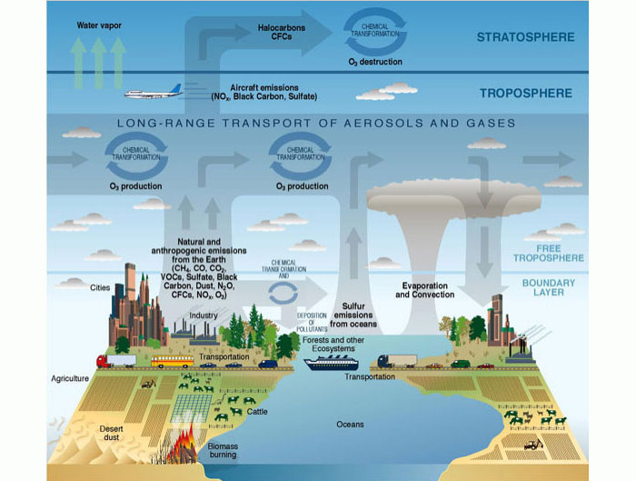
The science of air pollution centers on measuring, tracking, and predicting concentrations of key chemicals in the atmosphere. Four types of processes affect air pollution levels (Fig. 2):
- Emissions. Chemicals are emitted to the atmosphere by a range of sources. Anthropogenic emissions come from human activities, such as burning fossil fuels. Biogenic emissions are produced by natural functions of biological organisms, such as the microbial breakdown of organic materials. Emissions can also come from nonliving natural sources, most notably volcanic eruptions, and desert dust.
- Chemistry. Many types of chemical reactions in the atmosphere create, modify, and destroy chemical pollutants. These processes are discussed in the following sections.
- Transport. Winds can carry pollutants far from their sources so that emissions in one region cause environmental impacts far away. Long-range transport complicates efforts to control air pollution because it can be hard to distinguish effects caused by local versus distant sources and to determine who should bear the costs of reducing emissions.
- Deposition. Materials in the atmosphere return to Earth, either because they are directly absorbed or taken up in a chemical reaction (such as photosynthesis) or because they are scavenged from the atmosphere and carried to Earth by rain, snow, or fog.

Figure 2. Processes related to atmospheric composition
Source: Courtesy the United States Climate Change Science Program (Illustrated by P. Rekacewicz).
Air pollution trends are strongly affected by atmospheric conditions such as temperature, pressure, and humidity, and by global circulation patterns. For example, winds carry some pollutants far from their sources across national boundaries and even across the oceans. Transport is fastest along east-west routes: longitudinal winds can move air around the globe in a few weeks, compared to months or longer for air exchanges from north to south (for more details see Unit 2, “Atmosphere”).
Local weather patterns also interact with and affect air pollution. Rain and snow carry atmospheric pollutants to Earth. Temperature inversions, like the conditions that caused London’s Great Smog in 1952, occur when the air near the Earth’s surface is colder than air aloft. Cold air is heavier than warm air, so temperature inversions limit vertical mixing and trap pollutants near Earth’s surface. Such conditions are often found at night and during the winter months. Stagnation events characterized by weak winds are frequent during summer and can lead to the accumulation of pollutants over several days.
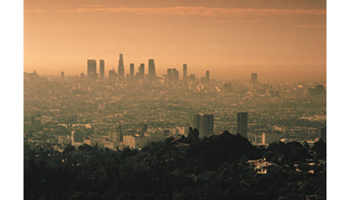
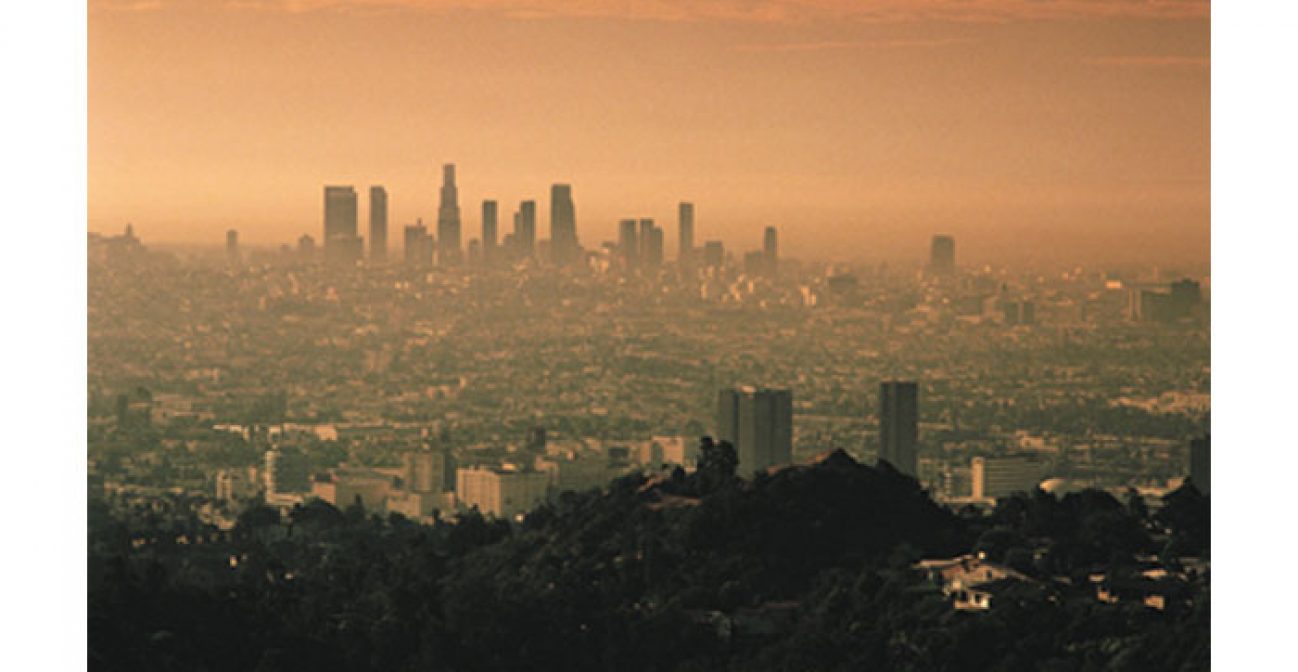
To see the close connections between weather, climate, and air pollution, consider Los Angeles, whose severe air quality problems stem partly from its physical setting and weather patterns. Los Angeles sits in a bowl, ringed by mountains to the north and east that trap pollutants in the urban basin. In warm weather, cool sea breezes are drawn onshore at ground level, creating temperature inversions that prevent pollutants from rising and dissipating. The region’s diverse manufacturing and industrial emitters and millions of cars and trucks produce copious primary air pollutants that mix in its air space to form photochemical smog (Fig. 3).

Figure 3. Smog over Los Angeles
Source: Courtesy the United States Environmental Protection Agency.
Scientists can measure air pollutants directly when they are emitted—for example, by placing instruments on factory smokestacks—or as concentrations in the ambient outdoor air. To track ambient concentrations, researchers create networks of air-monitoring stations, which can be ground-based or mounted on vehicles, balloons, airplanes, or satellites.
In the laboratory, scientists use tools including laser spectrometers and electron microscopes to identify specific pollutants. They measure chemical reaction rates in clear plastic bags (“smog chambers”) that replicate the smog environment under controlled conditions and observe emission of pollutants from combustion and other sources.
Knowledge of pollutant emissions, chemistry, and transport can be incorporated into computer simulations (“air quality models”) to predict how specific actions, such as requiring new vehicle emission controls or cleaner-burning fuels, will benefit ambient air quality. However, air pollutants pass through many complex reactions in the atmosphere and their residence times vary widely, so it is not always straightforward to estimate how emission reductions from specific sources will impact air quality over time.
3. Primary Air Pollutants
Unit 11 // Section 3
Primary air pollutants are emitted directly into the air from sources. They can have effects both directly and as precursors of secondary air pollutants (chemicals formed through reactions in the atmosphere), which are discussed in the following section.
Sulfur dioxide (SO2) is a gas formed when sulfur is exposed to oxygen at high temperatures during fossil fuel combustion, oil refining, or metal smelting. SO2 is toxic at high concentrations, but its principal air pollution effects are associated with the formation of acid rain and aerosols. SO2 dissolves in cloud droplets and oxidizes to form sulfuric acid (H2SO4), which can fall to Earth as acid rain or snow or form sulfate aerosol particles in the atmosphere. Associated impacts are discussed below in Section 5, “Aerosols,” and Section 7, “Acid Deposition.”
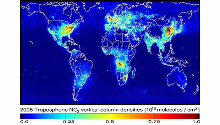
Nitrogen oxides (NO and NO2, referred together as NOx) are highly reactive gases formed when oxygen and nitrogen react at high temperatures during combustion or lightning strikes. Nitrogen present in fuel can also be emitted as NOx during combustion. Emissions are dominated by fossil fuel combustion at northern mid-latitudes and by biomass burning in the tropics. Figure 4 shows the distribution of NOx emissions to the atmosphere in 2006 as determined by satellite measurements of atmospheric NO2 concentrations.
In the atmosphere, NOx reacts with volatile organic compounds (VOCs) and carbon monoxide to produce ground-level ozone through a complicated chain reaction mechanism. It is eventually oxidized to nitric acid (HNO3). Like sulfuric acid, nitric acid contributes to acid deposition and aerosol formation.

Figure 4. Satellite observations of tropospheric NO2, 2006
Source: Courtesy Jim Gleason, USA and Pepijn Veefkind, KNMI, National Aeronautics, and Space Administration.
Carbon monoxide (CO) is an odorless, colorless gas formed by incomplete combustion of carbon in the fuel. The main source is motor vehicle exhaust, along with industrial processes and biomass burning. Carbon monoxide binds to hemoglobin in red blood cells, reducing their ability to transport and release oxygen throughout the body. Low exposures can aggravate cardiac ailments, while high exposures cause central nervous system impairment or death. It also plays a role in the generation of ground-level ozone, discussed below in Section 4.
[tootltip]Volatile organic compounds[/tootlip] (VOCs), including hydrocarbons (CxHy) but also other organic chemicals are emitted from a very wide range of sources, including fossil fuel combustion, industrial activities, and natural emissions from vegetation and fires. Some anthropogenic VOCs such as benzene are known carcinogens.
VOCs are also of interest as chemical precursors of ground-level ozone and aerosols, as discussed below in Sections 4 and 5. The importance of VOCs as precursors depends on their chemical structure and atmospheric lifetime, which can vary considerably from compound to compound. Large VOCs oxidize in the atmosphere to produce nonvolatile chemicals that condense to form aerosols. Short-lived VOCs interact with NOx to produce high ground-level ozone in polluted environments. Methane (CH4), the simplest and most long-lived VOC, is of importance both as a greenhouse gas (Section 11) and as a source of background tropospheric ozone. Major anthropogenic sources of methane include natural gas production and use, coal mining, livestock, and rice paddies.
4. Secondary Air Pollutants
Unit 11 // Section 4
Secondary pollutants form when primary pollutants react in the atmosphere. Table 1 summarizes common forms of atmospheric reactions.
| Type of reaction | Process | Notation |
|---|---|---|
| Bimolecular | Two reactants combine to produce two products. | A + B → C + D |
| Three-body | Two reactants combine to form one new product. A third, inert molecule (M) stabilizes the end product and removes excess energy. | A + B + M → AB + M |
| Photolysis | Solar radiation photon breaks a chemical bond in a molecule | A + hν → B + C |
| Thermal decomposition | A molecule decomposes by collision with an inert molecule (M) | A + M → B + C |
For reactions to take place, molecules have to collide. However, gases are present in the atmosphere at considerably lower concentrations than are typical for laboratory experiments or industrial processes, so molecules collide fairly infrequently. As a result, most atmospheric reactions that occur at significant rates involve at least one radical—a molecule with an odd number of electrons and hence an unpaired electron in its outer shell. The unpaired electron makes the radical unstable and highly reactive with other molecules. Radicals are formed when stable molecules are broken apart, a process that requires large amounts of energy. This can take place in combustion chambers due to high temperatures, and in the atmosphere by photolysis:
Nonradical + hν → radical + radical
Radical formation initiates reaction chains that continue until radicals combine with other radicals to produce nonradicals (atoms with an even number of electrons). Radical-assisted chain reactions in the atmosphere are often referred to as photochemical mechanisms because sunlight plays a key role in launching them.
One of the most important radicals in atmospheric chemistry is the hydroxyl radical(OH), sometimes referred to as the atmospheric cleanser. OH is produced mainly through photolysis reactions that break apart tropospheric ozone, and is very short-lived. It is consumed within about one second by oxidizing several trace gases like carbon monoxide, methane, and nonmethane VOCs (NMVOCs). Some of these reactions eventually regenerate OH in continuous cycles, while others deplete it.
Since OH has a short atmospheric lifetime, its concentration can vary widely. Some anthropogenic emissions, such as carbon monoxide and VOCs, deplete OH, while others such as NOx boost OH levels. Measuring atmospheric OH is difficult because its concentration is so low. Long-term trends in OH concentrations are uncertain, although the prevailing view is that trends over the past decades have been weak because of compensating influences from carbon monoxide and VOCs on the one hand and NOx on the other hand. Since OH affects the rates at which some pollutants are formed and others are destroyed, changes in OH levels over the long term would have serious implications for air quality.
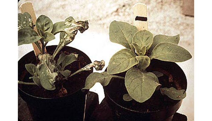
Ground-level ozone (O3) is a pernicious secondary air pollutant, toxic to both humans and vegetation (Fig. 5). It is formed in surface air (and more generally in the troposphere) by oxidation of VOCs and carbon monoxide in the presence of NOx. The mechanism is complicated, involving hundreds of chemically interactive species to describe the VOC degradation pathways. A simple schematic is:
VOC + OH → HO2 + other products
HO2 + NO → OH + NO2
NO2 + hν → NO + O
O + O2 + M → O3+ M
An important aspect of this mechanism is that NOx and OH act as catalysts—that is, they speed up the rate of ozone generation without being consumed themselves. Instead, they cycle rapidly between NO and NO2, and between OH and HO2.

Figure 5. Ozone damage to plant leaves
Source: Courtesy the United States Environmental Protection Agency.
This formation mechanism for ozone at ground level is different from that for ozone formation in the stratosphere, where 90 percent of total atmospheric ozone resides and plays a critical role in protecting life on Earth by providing a UV shield (for details see Unit 2, “Atmosphere”). In the stratosphere, ozone is produced from the photolysis of oxygen (O2 + hν → O + O, followed by O + O2 + M → O3 + M). This process does not take place in the troposphere because the strong (< 240 nm) UV photons needed to dissociate molecular oxygen are depleted by the ozone overhead.
5. Aerosols
Unit 11 // Section 5
In addition to gases, the atmosphere contains solid and liquid particles that are suspended in the air. These particles are referred to as aerosols or particulate matter (PM). Aerosols in the atmosphere typically measure between 0.01 and 10 micrometers in diameter, a fraction of the width of a human hair (Fig. 6). Most aerosols are found in the lower troposphere, where they have a residence time of a few days. They are removed when rain or snow carries them out of the atmosphere or when larger particles settle out of suspension due to gravity.

Figure 6. Size comparisons for aerosol pollution
Source: Courtesy United States Environmental Protection Agency.
Large aerosol particles (usually 1 to 10 micrometers in diameter) are generated when winds blow sea salt, dust, and other debris into the atmosphere. Fine aerosol particles with diameters less than 1 micrometer are mainly produced when precursor gases condense in the atmosphere. Major components of fine aerosols are sulfate, nitrate, organic carbon, and elemental carbon. Sulfate, nitrate, and organic carbon particles are produced by atmospheric oxidation of SO2, NOx, and VOCs as discussed above in Section 3. Elemental carbon particles are emitted by combustion, which is also a major source of organic carbon particles. Light-absorbing carbon particles emitted by combustion are called black carbon or soot; they are important agents for climate change and are also suspected to be particularly hazardous for human health.
High concentrations of aerosols are a major cause of cardiovascular disease and are also suspected to cause cancer. Fine particles are especially serious threats because they are small enough to be absorbed deeply into the lungs, and sometimes even into the bloodstream. Scientific research into the negative health effects of fine particulate air pollution spurred the U.S. Environmental Protection Agency to set limits in 1987 for exposure to particles with a diameter of 10 micrometers or less, and in 1997 for particles with a diameter of 2.5 micrometers or less.
Aerosols also have important radiative effects in the atmosphere. Particles are said to scatter light when they alter the direction of radiation beams without absorbing radiation. This is the principal mechanism limiting visibility in the atmosphere, as it prevents us from distinguishing an object from the background. Air molecules are inefficient scatterers because their sizes are orders of magnitude smaller than the wavelengths of visible radiation (0.4 to 0.7 micrometers). Aerosol particles, by contrast, are efficient scatterers. When relative humidity is high, aerosols absorb water, which causes them to swell and increases their cross-sectional area for scattering, creating haze. Without aerosol pollution, our visual range would typically be about 200 miles, but haze can reduce visibility significantly. Figure 7 shows two contrasting views of Acadia National Park in Maine on relatively good and bad air days.
Aerosols have a cooling effect on Earth’s climate when they scatter solar radiation because some of the scattered light is reflected into space. As discussed in Unit 12, “Earth’s Changing Climate,” major volcanic eruptions that inject large quantities of aerosols into the stratosphere, such as that of Mt. Pinatubo in 1991, can noticeably reduce average global surface temperatures for some time afterward.
In contrast, some aerosol particles such as soot absorb radiation and have a warming effect. This means that estimating the net direct contribution to global climate change from aerosols requires detailed inventories of the types of aerosols in the atmosphere and their distribution around the globe. Aerosol particles also influence Earth’s climate indirectly: they serve as condensation nuclei for cloud droplets, increasing the amount of radiation reflected into space by clouds and modifying the ability of clouds to precipitate. The latter is the idea behind “cloud seeding” in desert areas, where specific kinds of mineral aerosol particles that promote ice formation are injected into a cloud to make it precipitate.
Aerosol concentrations vary widely around the Earth (Fig. 8). Measurements are tricky because the particles are difficult to collect without modifying their composition. Combined optical and mass spectrometry techniques that analyze the composition of single particles directly in airflow, rather than recovering a bulk composition from filters, have improved scientists’ ability to detect and characterize aerosols (footnote 1).

Figure 8. Total ozone mapping spectrometer (TOMS) aerosol index of smoke and dust absorption, 2004
Source: Courtesy Jay Herman, NASA Goddard Space Flight Center.
One important research challenge is learning more about organic aerosols, which typically account for a third to half of the total aerosol mass. These include many types of carbon compounds with diverse properties and environmental impacts. Organic aerosols are emitted to the atmosphere directly by inefficient combustion. Automobiles, wood stoves, agricultural fires, and wildfires are major sources in the United States. Atmospheric oxidation of VOCs, both anthropogenic and biogenic, is another major source in summer. The relative importance of these different sources is still highly uncertain, which presently limits our ability to assess the anthropogenic influence and develop strategies for reducing concentrations.
6. Smog
Unit 11 // Section 6
Smog is often used as a generic term for any kind of air pollution that reduces visibility, especially in urban areas. However, it is useful to distinguish two broad types: industrial smog and photochemical smog.
Events like the London smog of 1952 are often referred to as industrial smog because SO2 emissions from burning coal play a key role. Typically, industrial smog—also called gray or black smog—develops under cold and humid conditions. Cold temperatures are often associated with inversions that trap the pollution near the surface (see Section 2, “Chemicals in Motion,” above). High humidity allows for rapid oxidation of SO2 to form sulfuric acid and sulfate particles. Events similar to the 1952 London smog occurred in the industrial towns of Liege, Belgium, in 1930, killing more than 60 people, and Donora, Pennsylvania, in 1948, killing 20. Today coal combustion is a major contributor to urban air pollution in China, especially from emissions of SO2 and aerosols (footnote 2).
Air pollution regulations in developed countries have reduced industrial smog events, but photochemical smog remains a persistent problem, largely driven by vehicle emissions. Photochemical smog forms when NOx and VOCs react in the presence of solar radiation to form ozone. The solar radiation also promotes the formation of secondary aerosol particles from the oxidation of NOx, VOCs, and SO2. Photochemical smog typically develops in summer (when solar radiation is strongest) in stagnant conditions promoted by temperature inversions and weak winds. Photochemical smog is a ubiquitous urban problem in the developed world and often blankets largely populated regions such as the eastern United States and western Europe for extended periods in summer.
Ozone and aerosols are the two main health hazards of photochemical smog. Ozone is invisible, but aerosol particles scatter sunlight as discussed above in Section 5, and are responsible for the whitish haze associated with smog. Because ozone is created in the atmosphere, concentrations are often higher downwind of urban areas than in the urban areas themselves. Figure 9 shows counties in the United States that currently fail to comply with the national standard for ozone levels over 8 hours (nonattainment areas). These cover much of California and the eastern United States on a regional scale.
 Figure 9. Nonattainment and maintenance areas in the U.S. 8-hour ozone standard
Source: Courtesy of the United States Environmental Protection Agency.
7. Acid Deposition
Unit 11 // Section 7
Acid rain[/tootlitp] was first identified in the 19th century when English pharmacist Robert Angus Smith measured high acidity levels in rain falling over industrial regions of England and much lower levels in less-polluted areas near the coast. However, this pattern did not receive sustained attention until biologists began to notice sharp declines in fish populations in lakes in Norway, the northeastern United States, and Canada in the 1950s and 1960s. In each case, researchers found that acid precipitation was altering lake chemistry. These findings spurred research into the causes of acid rain.
Pure water has a pH value of 7 (neutral), but rainwater falling in the atmosphere always contains impurities. The atmosphere contains natural acids including CO2 (a weak acid); nitric acid produced naturally from NOx emitted by lightning, fires, and soils; and sulfuric acid produced by the oxidation of sulfur gases from volcanoes and the biosphere. It also contains natural bases, including ammonia (NH3) emitted by the biosphere and calcium carbonate (CaCO3) from suspended soil dust. CO2 alone at natural levels (280 parts per million volume) would result in a rain pH of 5.7. Taken together, natural contaminants produce natural rain with pH values ranging from about 5 to 7 (recall that the pH scale is logarithmic, so one pH unit represents a factor of 10 difference in acid H+ concentration).
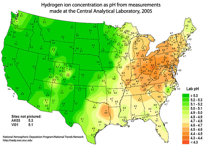
Acid rain refers to precipitation with pH values below 5, which generally happens only when large amounts of manmade pollution are added to the atmosphere. As Figure 10 shows, acid deposition takes place throughout the eastern United States and is particularly severe in the industrial Midwest due to its concentration of coal-burning power plants. Tall power plant stacks built to protect local air quality inject SO2 and NOx at high altitudes where winds are strong, allowing acid rain to extend more than a thousand miles downwind and into Canada.
 Figure 10. Hydrogen ion concentration
Source: Courtesy National Atmospheric Deposition Program/National Trends Network
The main components of acid rain worldwide are sulfuric acid and nitric acid. As discussed above in Section 3, these acids form when SO2 and NOx are oxidized in the atmosphere. Sulfuric and nitric acids dissolve in cloud water and dissociate to release H+:
HNO3 (aq) → NO3 – + H+
H2SO4(aq) → SO4 2- + 2H+
Human activity also releases large amounts of ammonia to the atmosphere, mainly from agriculture, and this ammonia can act as a base in the atmosphere to neutralize acid rain by converting H+ to the ammonium ion (NH4 +). However, the benefit of this neutralization is illusory because NH4 + releases its H+ once it is deposited and consumed by the biosphere. The relatively high pH of precipitation in the western United States is due in part to ammonia from agriculture and in part to suspended calcium carbonate (limestone) dust.
Acid rain has little effect on the environment in most of the world because it is quickly neutralized by naturally present bases after it falls. For example, the ocean contains a large supply of carbonate ions (CO3 2-), and many land regions have alkaline soils and rocks such as limestone. But in areas with little neutralizing capacity acid rain causes serious damage to plants, soils, streams, and lakes. In North America, the northeastern United States and eastern Canada are especially sensitive to acid rain because they have thin soils and granitic bedrock, which cannot neutralize acidity.
High acidity in lakes and rivers corrodes fishes’ organic gill material and attacks their calcium carbonate skeletons. Figure 11 shows the acidity levels at which common freshwater organisms can live and reproduce successfully. Acid deposition also dissolves toxic metals such as aluminum in soil sediments, which can poison plants and animals that take the metals up. And acid rain increases leaching of nutrients from forest soils, which weakens plants and reduces their ability to weather other stresses such as droughts, air pollution, or bug infestation.
 Figure 11. Acid tolerance ranges of common freshwater organisms
Source: Courtesy United States Environmental Protection Agency.
In addition to making ecosystems more acidic, deposition of nitrate and ammonia fertilizes ecosystems by providing nitrogen, which can be directly taken up by living organisms. Nitrogen pollution in rivers and streams is carried to the sea, where it contributes to algal blooms that deplete dissolved oxygen in coastal waters. As discussed in Unit 8, “Water Resources,” nutrient overloading has created dead zones in coastal regions around the globe, such as the Gulf of Mexico and the Chesapeake Bay. The main sources of nutrient pollution are agricultural runoff and atmospheric deposition.
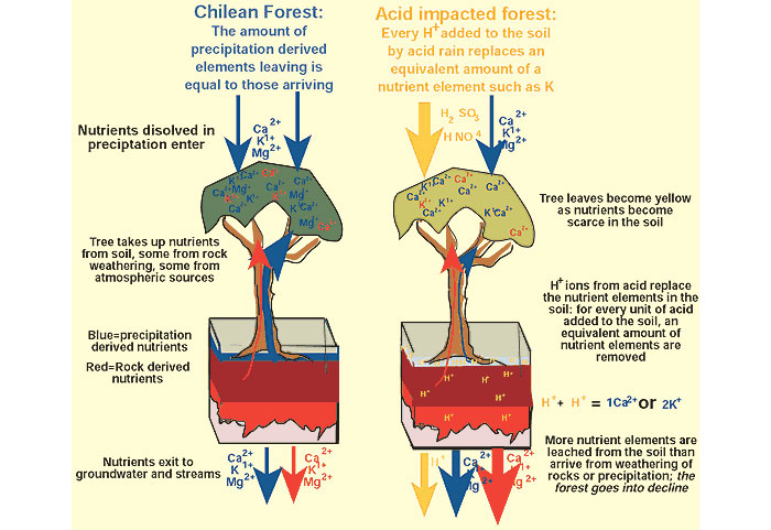
Acid rain levels have decreased and acid rain impacts have stabilized in the United States since SO2 and NOx pollution controls were tightened in 1990 (see Section 12, “Major Laws and Treaties,” below). However, acid deposition is in large part a cumulative problem, as the acid-neutralizing capacity of soils is gradually eroded in response to acid input, and eventual exhaustion of this acid-neutralizing capacity is a trigger for dramatic ecosystem impacts. A continued decrease in acid input is therefore critical. Figure 12 compares nutrient cycling in a pristine Chilean forest and a forest impacted by acid deposition.

Figure 12. Impact of acid rain on forest nutrient cycles
Source: © Martin Kennedy, University of California-Riverside.
8. Mercury Deposition
Unit 11 // Section 8
Mercury (Hg) is a toxic pollutant whose input to ecosystems has greatly increased over the past century due to anthropogenic emissions to the atmosphere and subsequent deposition. Mercury is ubiquitous in the environment and is unique among metals in that it is highly volatile. When materials containing mercury are burned, as in coal combustion or waste incineration, mercury is released to the atmosphere as a gas either in elemental form, Hg(0) or oxidized divalent form, Hg2+. The oxidized form is present as water-soluble compounds such as HgCl2 that are readily deposited in the region of their emission. By contrast, Hg(0) is not water-soluble and must be oxidized to Hg2+ to be deposited. This oxidation takes place in the atmosphere on a time scale of one year, sufficiently long that mercury can be readily transported around the world by atmospheric circulation. Mercury thus is a global pollution problem.
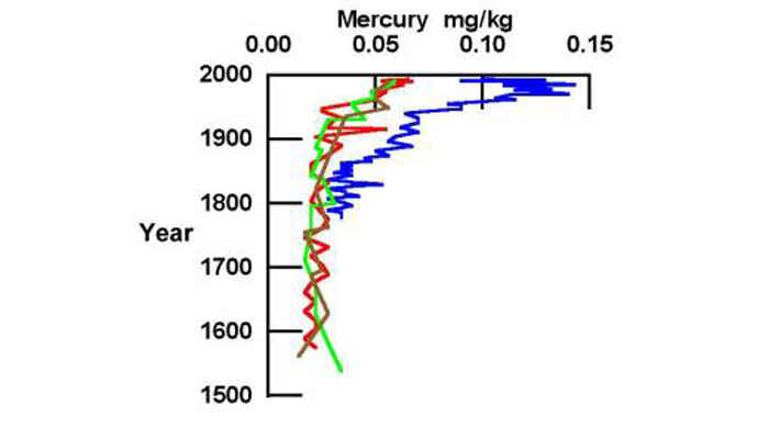
The deposition of anthropogenically emitted mercury to land and ocean has considerably raised mercury levels in the biosphere. This accumulation is evident from sediment cores that provide historical records of mercury deposition for the past several centuries (Fig. 13). Ice core samples from Antarctica, Greenland, and the western United States indicate that pre-industrial atmospheric mercury concentrations ranged from about 1 to 4 nanograms per liter, but that concentrations over the past 150 years have reached as high as 20 ng/L. (footnote 3)
 Figure 13. Mercury in sediment profiles from straits south of Norway
Source: Courtesy United Nations Environment Programme (adapted from Geological Survey of Norway).
Once deposited, oxidized mercury can be converted back to the elemental form Hg(0) and re-emitted to the atmosphere. This repeated re-emission is called the “grasshopper effect,” and can extend the environmental legacy of mercury emissions to several decades. The efficacy of re-emission increases with increasing temperature, which makes Hg(0) more volatile. As a result, mercury tends to accumulate to particularly high levels in cold regions such as the Arctic where re-emission is slow.
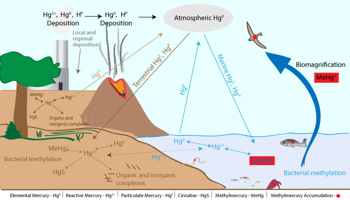
Divalent mercury deposited to ecosystems can be converted by bacteria to organic methylmercury, which is absorbed easily during digestion and accumulates in living tissues. It also enters fishes’ bodies directly through their skin and gills (Fig. 14). U.S. federal agencies and several states have issued warnings against consuming significant quantities of large predatory fish species such as shark and swordfish, especially for sensitive groups such as young children and women of childbearing age (footnote 4).

Figure 14. Conceptual biogeochemical mercury cycle
Mercury interferes with the brain and central nervous system. The expression “mad as a hatter” and the Mad Hatter character in Lewis Carroll’s Alice in Wonderland are based on symptoms common among 19th-century English hat makers, who inhaled mercury vapors when they used a mercurous nitrate solution to cure furs. Many hatters developed severe muscle tremors, distorted speech, and hallucinations as a result. Sixty-eight people died and hundreds were made ill or born with neurological defects in Minamata, Japan in the 1950s and 1960s after a chemical company dumped mercury into Minamata Bay and families ate fish from the bay. Recently, doctors have reported symptoms including dizziness and blurred vision in healthy patients who ate significant quantities of high-mercury fish such as tuna (footnote 5).
Developed countries in North America and Europe are largely responsible for the global build-up of mercury in the environment over the past century. They have begun to decrease their emissions over the past two decades in response to the recognized environmental threat. However, emissions in Asia have been rapidly increasing and it is unclear how the global burden of mercury will evolve over the coming decades. Because mercury is transported on a global scale, its control requires a global perspective. Also, the legacy of past emissions through re-emission and mercury accumulation in ecosystems must be recognized.
9. Controlling Air Pollution
Unit 11 // Section 9
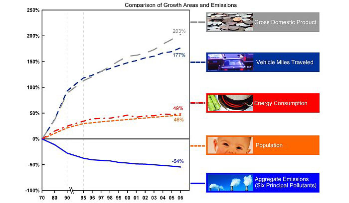
Thanks to several decades of increasingly strict controls, emissions of most major air pollutants have declined in the U.S. and other industrialized countries since the 1970s. Figure 15 shows the aggregate decrease in U.S. emissions since 1970. This trend occurred even as economic activity and fuel consumption increased. The reductions came about because governments passed laws limiting allowable pollution levels and required the use of technologies to reduce emissions, such as scrubbers on power plant smokestacks and catalytic converters on vehicles.

Figure 15. U.S. Economic Growth and Criteria Pollutant Emissions, 1970-2006
Source: Courtesy United States Environmental Protection Agency.
This decrease in emissions has demonstrably reduced levels of the four principal primary pollutants: carbon monoxide, nitrogen dioxide, sulfur dioxide, and lead. Air quality standards for these four pollutants were frequently exceeded in the U.S. twenty years ago but are hardly ever exceeded now.
Progress in reducing the two principal secondary pollutants, ozone, and particulate matter, has been much slower. This is largely due to nonlinear chemistry involved in the generation of these pollutants: reducing precursor emissions by a factor of two does not guarantee a corresponding factor of two decrease in the pollutant concentrations (the decrease is often much less, and there can even be an increase). Also, advances in health-effects research have generated constant pressure for tougher air quality standards for ozone and fine aerosols.
In contrast to improvements in developed countries, air pollution has been worsening in many industrializing nations. Beijing, Mexico City, Cairo, Jakarta, and other megacities in developing countries have some of the dirtiest air in the world (for more on environmental conditions in megacities, see Unit 5, “Human Population Dynamics”). This situation is caused by rapid population growth combined with rising energy demand, weak pollution control standards, dirty fuels, and inefficient technologies. Some governments have started to address this problem—for example, China is tightening motor vehicle emission standards—but much stronger actions will be required to reduce the serious public health impacts of air pollution worldwide.
10. Stratospheric Ozone
Unit 11 // Section 10
Earth’s stratospheric ozone layer, which contains about 90 percent of the ozone in the atmosphere, makes the planet habitable by absorbing harmful solar ultraviolet (UV) radiation before it reaches the planet’s surface. UV radiation damages cells and causes sunburn and premature skin aging in low doses. At higher levels, it can cause skin cancer and immune system suppression. Earth’s stratospheric ozone layer absorbs 99 percent of incoming solar UV radiation.
Scientists have worked to understand the chemistry of the ozone layer since its discovery in the 1920s. In 1930 British geophysicist Sydney Chapman described a process in which strong UV photons photolyze oxygen molecules (O2) into highly reactive oxygen atoms. These atoms rapidly combine with O2 to form ozone (O3) (Fig. 16). This process is still recognized as the only significant source of ozone to the stratosphere. Research and controversy have focused on identifying stratospheric ozone sinks.
 Figure 16. Ozone production
Source: Courtesy National Aeronautics and Space Administration.
Ozone is produced by different processes in the stratosphere, where it is beneficial, and near the Earth’s surface in the troposphere, where it is harmful. The mechanism for stratospheric ozone formation, photolysis of O2, does not take place in the troposphere because the strong UV photons needed for this photolysis have been totally absorbed by O2 and ozone in the stratosphere. In the troposphere, by contrast, the abundance of VOCs promotes ozone formation by the mechanism described above in Section 4. Ozone levels in the stratosphere are 10 to 100 times higher than what one observes at Earth’s surface in the worst smog events. Fortunately, we are not there to breathe it, through the exposure of passengers in jet aircraft to stratospheric ozone has emerged recently as a matter of public health concern.
To explain observed stratospheric ozone concentrations, we need to balance ozone production and loss. The formation of ozone in the stratosphere is simple to understand, but the mechanisms for ozone loss are considerably more complicated. Ozone photolyzes to release O2 and O, but this is not an actual sink since O2 and O can just recombine to ozone. The main mechanism for ozone loss in the natural stratosphere is a catalytic cycle involving NOx radicals, which speed up ozone loss by cycling between NO and NO2 but are not consumed in the process.
The main source of NOx in the troposphere is combustion; in contrast, the main source in the stratosphere is oxidation of nitrous oxide (N2O), which is emitted ubiquitously by bacteria at the Earth’s surface. Nitrous oxide is inert in the troposphere and can, therefore, be transported up to the stratosphere, where much stronger UV radiation enables its oxidation. Nitrous oxide emissions have increased over the past century due to agriculture, but the rise has been relatively modest (from 285 to 310 parts per million by volume) and of little consequence for the ozone layer.
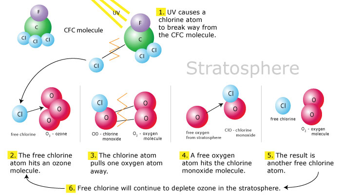
In 1974 chemists Sherwood Roland and Mario Molina identified a major threat to the ozone layer: rising atmospheric concentrations of manmade industrial chemicals called chlorofluorocarbons[/tootlitp] (CFCs), which at the time were widely used as refrigerants, in aerosol sprays, and in manufacturing plastic foams. CFC molecules are inert in the troposphere, so they are transported to the stratosphere, where they photolyze and release chlorine (Cl) atoms. Chlorine atoms cause catalytic ozone loss by cycling with ClO (Fig. 17).
 Figure 17. Chlorine-catalyzed ozone depletion mechanism
Eventually, chlorine radicals (Cl and ClO) are converted to the stable nonradical chlorine reservoirs of hydrogen chloride (HCl) and chlorine nitrate (ClNO3). These reservoirs slowly “leak” by oxidation and photolysis to regenerate chlorine radicals. Chlorine is finally removed when it is transported to the troposphere and washed out through deposition. However, this transport process is slow. Concern over chlorine-catalyzed ozone loss through the mechanism shown in Figure 17 led in the 1980s to the first measures to regulate the production of CFCs.
In 1985 scientists from the British Arctic Survey reported that springtime stratospheric ozone levels over their station at Halley Bay had fallen sharply since the 1970s. Global satellite data soon showed that stratospheric ozone levels were decreasing over most of the southern polar latitudes. This pattern, widely referred to as the “ozone hole” (more accurately, ozone thinning), proved to be caused by high chlorine radical concentrations, as well as by bromine radicals (Br), which also trigger catalytic cycles with chlorine to consume ozone.
The source of the high chlorine radicals was found to be a fast reaction of the chlorine reservoirs HCl and ClNO3 at the surface of icy particles formed at the very cold temperatures of the Antarctic wintertime stratosphere and called polar stratospheric clouds (PSCs). HCl and ClNO3 react on PSC surfaces to produce molecular chlorine (Cl2) and nitric acid. Cl2 then rapidly photolyzes in spring to release chlorine atoms and trigger ozone loss.
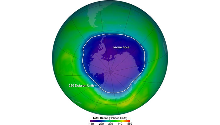
Ozone depletion has worsened since 1985. Today springtime ozone levels over Antarctica are less than half of the levels recorded in the 1960s, and the 2006 Antarctic ozone hole covered 29 million square kilometers, tying the largest value previously recorded in 2000 (Fig. 18). In the 1990s ozone loss by the same mechanism was discovered in the Arctic springtime stratosphere, although Arctic ozone depletion is not as extensive as in Antarctica because temperatures are not as consistently cold.

Figure 18. Antarctic ozone hole, October 4, 2004
Source: Courtesy National Aeronautics and Space Administration.
Rowland and Molina’s warnings about CFCs and ozone depletion, followed by the discovery of the ozone hole, spurred the negotiation of several international agreements to protect the ozone layer, leading eventually to a worldwide ban on CFC production in 1996 (for details see Section 12, “Major Laws and Treaties,” below). CFCs have lifetimes in the atmosphere of 50-100 years, so it will take that long for past damage to the ozone layer to be undone.
The Antarctic ozone hole is expected to gradually heal over the next several decades, but the effects of climate change pose major uncertainties. Greenhouse gases are well known to cool the stratosphere (although they warm the Earth’s surface), and a gradual decrease in stratospheric temperatures have been observed over the past decades. Cooling of the polar stratosphere promotes the formation of PSCs and thus the release of chlorine radicals from chlorine reservoirs. The question now is whether the rate of decrease of stratospheric chlorine over the next decades will be sufficiently fast to stay ahead of the cooling caused by increasing greenhouse gases. This situation is being closely watched by atmospheric scientists both in Antarctica and the Arctic.
11. Air Pollution, Greenhouse Gases, and Climate Change
Unit 11 // Section 11
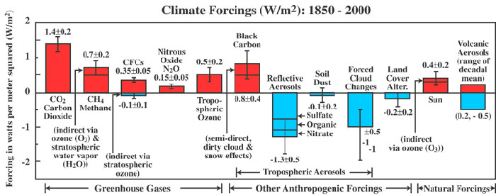
Air pollutants are major contributors to climate change. This connection is well known to scientists, although it has not yet permeated environmental policy. Figure 19 shows global climate forcing for the year 2000, relative to 1850, caused by different observed perturbations to the Earth system. Climate forcing from a given perturbation is defined as the mean resulting imbalance between energy input and energy output per unit time and unit area of Earth’s surface (watts per square meter or W/m2), with all else remaining constant, including temperature. A positive radiative forcing means a decrease in energy output and hence warming, shown as red bars in Fig. 19. Negative radiative forcing, shown as blue bars in Fig. 19, means a decrease in energy input and hence a cooling. (For more on climate forcing see Unit 12, “Earth’s Changing Climate.”)
Figure 19 shows that a large number of perturbation agents have forced the climate since 1850. CO2 is the single most important agent, but many other agents are also important and together exert greater influence than CO2.
 Figure 19. Climate forcings (W/m2): 1850–2000
Source: Courtesy James E. Hansen, NASA Goddard Institute for Space Studies.
Among the major greenhouse gases in Figure 19 are methane and tropospheric ozone, which are both of concern for air quality. Light absorption by black carbon aerosol particles also has a significant warming effect. Taken together these three agents produce more radiative forcing than CO2. Reductions in these air pollutants thus would reap considerable benefits for climate change.
However, air pollutants can also have a cooling effect that compensates for greenhouse warming. This factor can be seen in Figure 19 from the negative radiative forcings due to non-light-absorbing sulfate and organic aerosols originating from fossil fuel combustion. Scattering by these aerosols is estimated by the [tootltip]Intergovernmental Panel on Climate Change (IPCC)[/tooltip] to have a direct radiative forcing of -1.3 W/m2, although this figure is highly uncertain. Indirect radiative forcing from increased cloud reflectivity due to anthropogenic aerosols is even more uncertain but could be as large as -1 W/m2.
Scattering aerosols have thus masked a significant fraction of the warming imposed by increasing concentrations of greenhouse gases over the past two centuries. Aerosol and acid rain control policies, though undeniably urgent to protect public health and ecosystems, will reduce this masking effect and expose us to more greenhouse warming.
Influence also runs the other way. Global climate change has the potential to magnify air pollution problems by raising Earth’s temperature (contributing to tropospheric ozone formation) and increasing the frequency of stagnation events. Climate change is also expected to cause more forest fires and dust storms, which can cause severe air quality problems (Fig. 20).

Figure 20. Fire plumes over Southern California, October 26, 2003
Source: Courtesy National Aeronautics and Space Administration.
The link between air pollution and climate change argues for developing environmental policies that will yield benefits in both areas. For example, researchers at Harvard University, Argonne National Laboratory, and the Environmental Protection Agency estimated in 2002 that reducing anthropogenic methane emissions by 50 percent would not only reduce greenhouse warming but also nearly halve the number of high-ozone events in the United States. Moreover, since methane contributes to background ozone levels worldwide, this approach would reduce ozone concentrations globally. In contrast, reducing NOx emissions—the main U.S. strategy for combating ozone—produces more localized reductions to ozone (footnote 6).
Finally, let us draw the distinction between stratospheric ozone depletion and climate change since these two problems are often confused in the popular press. As summarized in Table 2, the causes, processes, and impacts of these two global perturbations to the Earth system are completely different, but they have some links. On the one hand, colder stratospheric temperatures due to increasing greenhouse gases intensify polar ozone loss by promoting PSC formation, as discussed in Section 9. On the other hand, CFCs are major greenhouse gases, and stratospheric ozone depletion exerts a slight cooling effect on the Earth’s surface.
| Ozone depletion | Global warming | |
|---|---|---|
| Location | Stratosphere | Troposphere (stratosphere actually cools) |
| Causative pollutant | Ozone-depleting substances (NOx, CFCs) | Greenhouse gases (CO2, CH4, N2O, tropospheric ozone) |
| Process | Catalytic ozone loss reactions | Trapping of infrared radiation emitted by Earth’s surface |
12. Major Laws and Treaties
Unit 11 // Section 12
The first international treaty to protect the ozone layer was signed in 1987. The [tootltip]Montreal Protocol on Substances That Deplete the Ozone Layer[/tooltip] has been amended several times since then in response to new scientific information, and it has been ratified by 190 countries. Under it, industrialized countries phased out the production of several classes of ozone-depleting substances by 1996, and developing countries are to follow suit by 2010. An international fund created under the protocol helps developing nations find substitutes for ozone-depleting substances. The World Bank estimates that reductions under the Montreal Protocol through 2003 have avoided up to 20 million cases of cancer, 130 million cases of eye cataracts, and severe damage to ecosystems from increased UV radiation reaching Earth’s surface (footnote 7).
When nations began to negotiate agreements on reducing greenhouse gases to slow global climate change, many experts believed that the problem could be addressed through a framework similar to the Montreal Protocol—a treaty that set timetables for phasing out harmful emissions, with technical aid to help developing countries comply. But climate change has proved to be a considerably harder problem for negotiators, for several reasons. These negotiations are discussed in Unit 12, “Earth’s Changing Climate.”
The Clean Air Act (CAA) sets out a comprehensive set of national standards for controlling air pollutants that are considered harmful to public health and the environment in the United States. Under the CAA the Environmental Protection Agency is directed to establish National Ambient Air Quality Standards (NAAQS) limiting major air pollutants to levels that will protect public health, including the health of sensitive groups such as children, the elderly, and people with respiratory illnesses. NAAQS are set based on input from scientific advisory committees, and the act specifically directs EPA not to consider costs in setting NAAQS, although states can consider costs when they develop their plans for meeting the standards.
EPA has established NAAQS for six “criteria pollutants”: SO2, NO2, lead, carbon monoxide, particulate matter less than 10 micrometers and less than 2.5 micrometers (PM-10 and PM-2.5), and ozone. States and counties that fail to achieve these standards are required to develop plans for bringing their air quality into compliance. The CAA also defines major pollution sources, based on their emission levels, and establishes rules governing when new emission sources can be built in polluted areas.
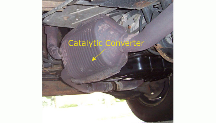
The CAA has been amended several times since its passage in 1970 to tighten standards and institute new controls that reflect advances in scientific understanding of air pollution. The law has achieved some notable successes: for example, it has reduced U.S. automobile emissions considerably from pre-1970 levels, through mechanisms such as phasing out the use of leaded gasoline and requiring car manufacturers to install catalytic converters. These devices treat car exhaust in several stages to reduce NOx and oxidize unburned hydrocarbons and carbon monoxide (Fig. 21).

Figure 21. Catalytic converter mounted in a car’s exhaust system
Source: Courtesy Wikimedia Commons. Public Domain.
A set of CAA amendments passed in 1990 has produced significant cuts in SO2emissions through what was then a new approach to reducing air pollution: capping the total allowable amount of pollution emitted nationally and then allocating emission rights among major sources (mainly coal-burning electric power plants and industrial facilities). Emitters that reduced pollution below their allowed levels could sell their extra pollution allowances to higher-emitting sources. This approach let sources make reductions where they were cheapest, rather than requiring all emitters to install specific pieces of control equipment or to meet one standard at each location. Some companies cut emissions by installing controls, while others switched to low-sulfur coal or other cleaner fuels.
U.S. SO2 emissions have fallen by roughly 50 percent since emissions trading was instituted, and the program is widely cited as an example of how this approach can work more effectively than technology mandates. However, some proposals for emissions trading are more controversial—specifically, whether it is a safe approach for cutting toxic pollutants such as mercury. Opponents argue that letting some large sources continue to emit such pollutants could create dangerous “hot spots” that would be hazardous to public health, and that the only safe way to control hazardous pollutants like mercury is to require specific reductions from each individual source.
13. Further Reading
Unit 11 // Section 13
Further Reading
C.T. Driscoll et al., Acid Rain Revisited: Advances in Scientific Understanding Since the Passage of the 1970 and 1990 Clean Air Act Amendments, Hubbard Brook Research Foundation, Science Links Publication, vol. 1. no. 1 (2001).
Daniel Jacob, Introduction to Atmospheric Chemistry (Princeton University Press, 1999). An overview of the field that shows how to use basic principles of physics and chemistry to describe a complex system such as the atmosphere.
Peter H. McMurry, Marjorie F. Shepherd, and James S. Vickery, eds., Particulate Matter Science for Policy Makers: A NARSTO Assessment (Cambridge University Press, 2004). Scientific information about particulate emissions and their impacts, produced by a North American consortium for atmospheric research in support of air quality management.
National Research Council, Air Quality Management in the United States (Washington, DC: National Academies Press, 2004). A Congressionally mandated study of how well major U.S. air quality laws have worked from a scientific and technical perspective, and ways in which they could be strengthened.
Footnotes
- Daniel M. Murphy, “Something in the Air,” Science, March 25, 2005, pp. 1888–1890.
- National Academies of Science, Urbanization, Energy, and Air Pollution in China: The Challenges Ahead (Washington, DC: National Academies Press, 2004), p. 3.
- U.S. Geological Survey, “Glacial Ice Cores Reveal A Record of Natural and Anthropogenic Atmospheric Mercury Deposition for the Last 270 Years,” June 2002, http://toxics.usgs.gov/pubs/FS-051-02/.
- For the latest version, see U.S. Environmental Protection Agency, “Fish Advisories,” http://www.epa.gov/waterscience/fish/.
- Jane M. Hightower and Dan Moore, “Mercury Levels in High-End Consumers of Fish,” Environmental Health Perspectives, Vol. 111., No. 4, April 2003, pp. 604–608; Eric Duhatschek, “Charity Games in Quebec Will Help Kids,” The Globe and Mail, October 8, 2004, p. R11.
- Arlene M. Fiore et al., “Linking Ozone Pollution and Climate Change: The Case for Controlling Methane,” Geophysical Research Letters, Vol. 29, No. 19 (2002), pp. 25–28.
- World Bank, “The World Bank and the Montreal Protocol,” September 2003, http://siteresources.worldbank.org/INTMP/214578-1110890369636/20489383/WBMontrealProtocolStatusReport2003.pdf.