The Fundamental Interactions Online Textbook

The underlying theory of the physical world has two fundamental components: Matter and its interactions. We examined the nature of matter in the previous unit. Now we turn to interactions, or the forces between particles. Just as the forms of matter we encounter on a daily basis can be broken down into their constituent fundamental particles, the forces we experience can be broken down on a microscopic level. We know of four fundamental forces: electromagnetism, gravity, the strong nuclear force, and the weak force.

Electromagnetism causes almost every physical phenomenon we encounter in our everyday life: light, sound, the existence of solid objects, fire, chemistry, all biological phenomena, and color, to name a few. Gravity is, of course, responsible for the attraction of all things on the Earth toward its center, as well as tides—due to the pull of the Moon and the Sun on the oceans—the motions within the solar system, and even the formation of large structures in the universe, such as galaxies. The strong force takes part in all nuclear phenomena, such as fission and fusion, the latter of which occurs at the core of our Sun and all other stars. Finally, the weak force is involved in radioactivity, causing unstable atomic nuclei to decay. The latter two operate only at microscopic distances, while the former two clearly have significant effects on macroscopic scales.

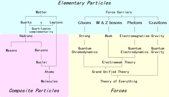
Figure 1: This chart shows the known fundamental particles—those of matter and those of force.
Source: © Wikimedia Commons, Creative Commons Attribution ShareAlike 3.0, Author: Headbomb, 21 January 2009.

In this unit, we will discover a number of the astounding unifying principles of particle physics: First, that forces themselves can be described as particles, too—force particles exchanged between matter particles. Then, that particles are not fundamental at all, which is why they can disappear and reappear at particle colliders. Next, that subatomic physics is best described by a new mathematical framework called quantum field theory (QFT), where the distinction between particle and force is no longer clear. And finally, that all four fundamental forces seem to operate under the same basic rules, suggesting a deeper unifying principle of all forces of Nature.

Many forms of force

How do we define a force? And what is special about the fundamental forces? We can start to answer those questions by observing the many kinds of forces at work in daily life—gravity, friction, “normal forces” that appear when a surface presses against another surface, and pressure from a gas, the wind, or the tension in a taut rope. While we normally label and describe these forces differently, many of them are a result of the same forces between atoms, just manifesting in different ways.

Figure 2: An example of conservative (right) and non-conservative (left) forces.
Source: © Left: Jon Ovington, Creative Commons Attribution-ShareAlike 2.0 Generic License. Right: Benjamin Crowell, lightandmatter.com, Creative Commons Attribution-ShareAlike 3.0 License.

At the macroscopic level, physicists sometimes place forces in one of two categories: conservative forces that exchange potential energy and kinetic energy, such as a sled sliding down a snowy hill; and non-conservative forces that transform kinetic energy into heat or some other dissipative type of energy. The former is characterized by its reversibility, and the latter by its irreversibility: It is no problem to push the sled back up the snowy hill, but putting heat back into a toaster won’t generate an electric current.

But what is force? Better yet, what is the most useful description of a force between two objects? It depends significantly on the size and relative velocity of the two objects. If the objects are at rest or moving much more slowly than the speed of light with respect to each other, we have a perfectly fine description of a static force. For example, the force between the Earth and Sun is given to a very good approximation by Newton’s law of universal gravitation, which only depends on their masses and the distance between them. In fact, the formulation of forces by Isaac Newton in the 17th century best describes macroscopic static forces. However, Newton did not characterize the rules of other kinds of forces beyond gravity. In addition, the situation gets more complicated when fundamental particles moving very fast interact with one another.

Forces at the microscopic level

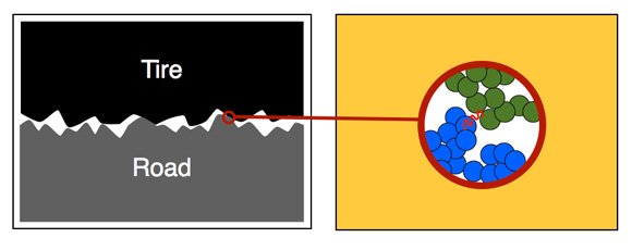
At short distances, forces can often be described as individual particles interacting with one another. These interactions can be characterized by the exchange of energy (and momentum). For example, when a car skids to a stop, the molecules in the tires are crashing into molecules that make up the surface of the road, causing them to vibrate more on the tire (i.e., heat up the tire) or to be ripped from their bonds with the tire (i.e., create skid marks).

A microscopic view of friction. © David Kaplan.

When conserving energy, however, one must take into account Einstein’s relativity—especially if the speeds of the particles are approaching the speed of light. For a particle in the vacuum, one can characterize just two types of energy: The energy of motion and the energy of mass. The latter, summarized in the famous equation E=mc², suggests that mass itself is a form of energy. However, Einstein’s full equation is more complicated. In particular, it involves an object’s momentum, which depends on the object’s mass and its velocity. This applies to macroscopic objects as well as those at the ultra-small scale. For example, chemical and nuclear energy is energy stored in the mass difference between molecules or nuclei before and after a reaction. When you switch on a flashlight, for example, it loses its mass to the energy of the photons leaving it—and actually becomes lighter! See Einstein’s Equation in The Math section below.

When describing interactions between fundamental particles at very high energies, it is helpful to use an approximation called the relativistic limit, in which we ignore the mass of the particles. In this situation, the momentum energy is much larger than the mass energy, and the objects are moving at nearly the speed of light. These conditions occur in particle accelerators. But they also existed soon after the Big Bang when the universe was at very high temperatures and the particles that made up the universe had large momenta. As we will explain later in this unit, we expect new fundamental forces of nature to reveal themselves in this regime. So, as in Unit 1, we will focus on high-energy physics as a way to probe the underlying theory of force.

A way to measure the fundamental forces between particles is by measuring the probability that the particles will scatter off each other when one is directed toward the other at a given energy. We quantify this probability as an effective cross-sectional area, or cross section, of the target particle. The concept of a cross-section applies in more familiar examples of scattering as well. For example, the cross-section of a billiard ball (See Figure 4) is the area at which the oncoming ball’s center has to be aimed in order for the balls to collide. In the limit that the white ball is infinitesimally small, this is simply the cross-sectional area of the target (yellow) ball.

The cross-section of a particle in an accelerator is similar conceptually. It is an effective size of the particle—like the size of the billiard ball—that not only depends on the strength and properties of the force between the scattering particles, but also on the energy of the incoming particles. The beam of particles comes in, sees the cross-section of the target, and some fraction of them scatter, as illustrated in the bottom of Figure 4. Thus, from a cross-section, and the properties of the beam, we can derive a probability of scattering.

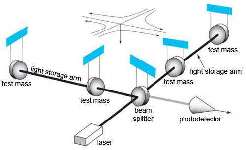
Figure 5: This movie shows the simplest way two electrons can scatter.
Source: © David Kaplan

The simplest way two particles can interact is to exchange some momentum. After the interaction, the particles still have the same internal properties but are moving at different speeds in different directions. This is what happens with the billiard balls, and is called “elastic scattering.” In calculating the elastic scattering cross-section of two particles, we can often make the approximation depicted in Figure 5. Here, the two particles move freely toward each other; they interact once at a single point and exchange some momentum, and then they continue on their way as free particles. The theory of the interaction contains information about the probabilities of momentum exchange, the interactions between the quantum mechanical properties of the two particles known as spins, and a dimensionless parameter, or coupling, whose size effectively determines the strength of the force at a given energy of an incoming particle.

Such an approximation, that the interaction between particles happens at a single point in space at a single moment in time, may seem silly. The force between a magnet and a refrigerator, for example, acts over a distance much larger than the size of an atom. However, when the particles in question are moving fast enough, this approximation turns out to be quite accurate—in some cases extremely so. This is in part due to the probabilistic nature of quantum mechanics, a topic treated in depth in Unit 5. When we are working with small distances and short times, we are clearly in the quantum mechanical regime.

We can approximate the interaction between two particles as the exchange of a new particle between them called a . One particle emits the force carrier and the other absorbs it. In the intermediate steps of the process—when the force carrier is emitted and absorbed—it would normally be impossible to conserve energy and momentum. However, the rules of quantum mechanics govern particle interactions, and those rules have a loophole.

The loophole that allows force carriers to appear and disappear as particles interact is called the Heisenberg uncertainty principle">force carrier. One particle emits the force carrier and the other absorbs it. In the intermediate steps of the process—when the force carrier is emitted and absorbed—it would normally be impossible to conserve energy and momentum. However, the rules of quantum mechanics govern particle interactions, and those rules have a loophole.

The loophole that allows force carriers to appear and disappear as particles interact is called the Heisenberg uncertainty principle. German physicist Werner Heisenberg outlined the uncertainty principle named for him in 1927. It places limits on how well we can know the values of certain physical parameters. The uncertainty principle permits a distribution around the “correct” or “classical” energy and momentum at short distances and over short times. The effect is too small to notice in everyday life, but becomes powerfully evident over the short distances and times experienced in high-energy physics. While the emission and absorption of the force carrier respect the conservation of energy and momentum, the exchanged force carrier particle itself does not. The force carrier particle does not have a definite mass and in fact doesn’t even know which particle emitted it and which absorbed it. The exchanged particles are unobservable directly, and thus are called virtual particles.

FEYNMAN, FINE PHYSICIST

Richard Feynman was a major contributor to field of physics. © AIP Emilio Segrè Visual Archives.

During a glittering physics career, Richard Feynman did far more than create the diagrams that carry his name. In his 20s, he joined the fraternity of atomic scientists in the Manhattan Project who developed the atom bomb. After World War II, he played a major role in developing quantum electrodynamics, an achievement that won him the Nobel Prize in physics. He made key contributions to understanding the nature of superfluidity and to aspects of particle physics. He has also been credited with pioneering the field of quantum computing and introducing the concept of nanotechnology.

Feynman’s contributions went beyond physics. As a member of the panel that investigated the 1986 explosion of the space shuttle Challenger, he unearthed serious misunderstandings of basic concepts by NASA’s managers that helped to foment the disaster. He took great interest in biology and did much to popularize science through books and lectures. Eventually, Feynman became one of the world’s most recognized scientists, and is considered the best expositor of complex scientific concepts of his generation.

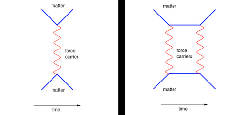
Physicists like to draw pictures of interactions like the ones shown in Figure 6. The left side of Figure 6, for example, represents the interaction between two particles through one-particle exchange. Named a Feynman diagram for American Nobel Laureate and physicist Richard Feynman, it does more than provide a qualitative representation of the interaction. Properly interpreted, it contains the instructions for calculating the scattering cross-section. Linking complicated mathematical expressions to a simple picture made the lives of theorists a lot easier.

Even more important, Feynman diagrams allow physicists to easily organize their calculations. It is in fact unknown how to compute most scattering cross-sections exactly (or analytically). Therefore, physicists make a series of approximations, dividing the calculation into pieces of decreasing significance. The Feynman diagram on the left side of Figure 6 corresponds to the first level of approximation—the most significant contribution to the cross-section that would be evaluated first. If you want to calculate the cross-section more accurately, you will need to evaluate the next most important group of terms in the approximation, given by diagrams with a single loop, like the one on the right side of Figure 6. By drawing every possible diagram with the same number of loops, physicists can be sure they haven’t accidentally left out a piece of the calculation.

Feynman diagrams are far more than simple pictures. They are tools that facilitate the calculation of how particles interact in situations that range from high-energy collisions inside particle accelerators to the interaction of the constituent parts of a single, trapped ion. As we will see in Unit 5, one of the most precise experimental tests of quantum field theory compares a calculation based on hundreds of Feynman diagrams to the behavior of an ion in a trap. For now, we will focus on the conceptually simpler interaction of individual particles exchanging a virtual force carrier.

Figure 6: Feynman diagram representing a simple scattering of two particles (left) and a more complicated scattering process involving two particles (right).
Source: © David Kaplan.

Figure 7: When an electron and its antiparticle collide, they annihilate and new particles are created.
Source: © David Kaplan.

At a particle collider, it is possible for an electron and an antielectron to collide at a very high energy. The particles annihilate each other, and then two new particles, a muon and an antimuon, come out of the collision. There are two remarkable things about such an event, which has occurred literally a million times at the LEP collider that ran throughout the 1990s at CERN. First, the muon is 200 times heavier than the electron. We see in a dramatic way that mass is not conserved—that the kinetic energy of the electrons can be converted into mass for the muon. E = mc², again. Mass is not a fundamental quantity.

The second remarkable thing is that particles like electrons and muons can appear and disappear, and thus they are, in some sense, not fundamental. In fact, all particles seem to have this property. Then what is fundamental? In response to this question, physicists define something called a field. A field fills all of space, and the field can, in a sense, vibrate in a way that is analogous to ripples on a lake. The places a field vibrates are places that contain energy, and those little pockets of energy are what we call (and have the properties of) particles.

As an analogy, imagine a lake. A pebble is dropped in the lake, and a wave from the splash travels away from the point of impact. That wave contains energy. We can describe that package of localized energy living in the wave as a particle. One can throw a few pebbles in the lake at the same time and create multiple waves (or particles). What is fundamental then is not the particle (wave), it is the lake itself (field). In addition, the wave (or particle) would have different properties if the lake were made of water or of, say, molasses. Different fields allow for the creation of different kinds of particles.

Figure 7: A circular wave created by tossing a pebble in a pond. Source: © Adam Kleppner.

To describe a familiar particle such as the electron in a quantum field theory, physicists consider the possible ways the electron field can be excited. Physicists say that an electron is the one-particle state of the electron field—a state well defined before the electron is ever created. The quantum field description of particles has one important implication: Every electron has exactly the same internal properties—the charge, spin, and mass for each electron exactly matches that for every other one. In addition, the symmetries inherent in relativity require that every particle has an antiparticle with opposite spin, electric charge, and other charges. Some uncharged particles, such as photons, act as their own antiparticles.

A crucial distinction

In general, the fact that all particles—matter or force carriers—are excitations of fields is the great unifying concept of quantum field theory. The excitations all evolve in time like waves, and they interact at points in spacetime like particles. However, the theory contains one crucial distinction between matter and force carriers. This relates to the internal spin of the particles.

By definition, all matter particles, such as electrons, protons, and neutrons, as well as quarks, come with a half-unit of spin. It turns out in quantum mechanics that a particle’s spin is related to its angular momentum, which, like energy and linear momentum, is a conserved quantity. While a particle’s linear momentum depends on its mass and velocity, its angular momentum depends on its mass and the speed at which it rotates about its axis. Angular momentum is quantized—it can take on values only in multiples of Planck’s constant , ħ = 1.05 x 10^-34Joule-seconds. So the smallest amount by which an object’s angular momentum can change is λ. This value is so small that we don’t notice it in normal life. However, it tightly restricts the physical states allowed for the tiny angular moment in atoms. Just to relate these amounts to our everyday experience, a typical spinning top can have an angular momentum of 1,000,000,000,000,000,000,000,000,000,000 times ħ. If you change the angular momentum of the top by multiples of ħ Now, force carriers all have integer units of internal spin; no fractions are allowed. When these particles are emitted or absorbed, their spin can be exchanged with the rotational motion of the particles, thus conserving angular momentum. Particles with half-integer spin cannot be absorbed, because the smallest unit of rotational angular momentum is one times ħ. Physicists call particles with half-integer spin fermions. Those with integer (including zero) spins they name bosons, you may as well be changing it continuously. This is why we don’t see the quantum-mechanical nature of spin in everyday life.

Not your grandmother’s ether theory

Figure 9: Experimental results remain the same whether they are performed at rest or at a constant velocity. Source: © David Kaplan.

An important quantum state in the theory is the “zero-particle state,” or vacuum. The fact that spacetime is filled with quantum fields makes the vacuum much more than inactive empty space. As we shall see later in this unit, the vacuum state of fields can change the mass and properties of particles. It also contributes to the energy of spacetime itself. But the vacuum of spacetime appears to be relativistic; in other words, it is best described by the theory of relativity. For example, in Figure 9, a scientist performing an experiment out in empty space will receive the same result as a scientist carrying out the same experiment while moving at a constant velocity relative to the first. So we should not compare the fields that fill space too closely with a material or gas. Moving through air at a constant velocity can affect the experiment because of air resistance. The fields, however, have no preferred “at rest” frame. Thus, moving relative to someone else does not give a scientist or an experiment a distinctive experience. This is what distinguishes quantum field theory from the so-called “ether” theories of light of a century ago.

The electromagnetic force dominates human experience. Apart from the Earth’s gravitational pull, nearly every physical interaction we encounter involves electric and/or magnetic fields. The electric forces we constantly experience have to do with the nature of the atoms we’re made of. Particles can carry electric charge, either positive or negative. Particles with the same electric charge repel one another, and particles with opposite electric charges attract each other. An atom consists of negatively charged electrons in the electric field of a nucleus, which is a collection of neutrons and positively charged protons. The negatively charged electrons are bound to the positively charged nucleus.

Figure 10: The electromagnetic force and the constituents of matter. All material we experience—solid, liquid, or anything in between—is held together by the electromagnetic force. While this glass of water may be essentially neutral, and has approximately the same number of positive and negative charges, the water is made of molecules, which are made of atoms, which are made of charged particles—protons and electrons. These particles not only attract each other within the atoms through the electromagnetic force, but from atom to atom, and molecule to molecule. The attractions and repulsions deform the atoms and molecules in such a way that the net result is an attraction between molecules, and thus macroscopic materials form. (Unit: 2)
Source: © David Kaplan.

Although atoms are electrically neutral, they can attract each other and bind together, partly because atoms do have oppositely charged component parts and partly due to the quantum nature of the states in which the electrons find themselves (see Unit 6). Thus, molecules exist owing to the electric force. The residual electric force from electrons and protons in molecules allows the molecules to join up in macroscopic numbers and create solid objects. The same force holds molecules together more weakly in liquids. Similarly, electric forces allow waves to travel through gases. Thus, sound is a consequence of electric force, and so are many other common phenomena, including electricity, friction, and car accidents.

We experience magnetic force from materials such as iron and nickel. At the fundamental level, however, magnetic fields are produced by moving electric charges, such as electric currents in wires, and spinning particles, such as electrons in magnetic materials. So, we can understand both electric and magnetic forces as the effects of classical electric and magnetic fields produced by charged particles acting on other charged particles.

The close connection between electricity and magnetism emerged in the 19th century. In the 1830s, English scientist Michael Faraday discovered that changing magnetic fields produced electric fields. In 1861, Scottish physicist James Clerk Maxwell postulated that the opposite should be true: A changing electric field would produce a magnetic field. Maxwell developed equations that seemed to describe all electric and magnetic phenomena. His solutions to the equations described waves of electric and magnetic fields propagating through space—at speeds that matched the experimental value of the speed of light. Those equations provided a unified theory of electricity, magnetism, and light, as well as all other types of electromagnetic radiation, including infrared and ultraviolet light, radio waves, microwaves, x-rays, and gamma rays.

Figure 11: Michael Faraday (left) and James Clerk Maxwell (right) unified electricity and magnetism in classical field theory. Michael Faraday (1791-1867, left) had little formal education in science or mathematics, but performed a tremendous series of experiments in electricity and magnetism in his laboratory in Scotland that teased out both the subtle features and basic laws of both phenomena. James Clerk Maxwell (1831-1879, right) provided the theoretical counterpart to Faraday’s experimental program. Maxwell synthesized numerous, disparate experimental results into a coherent theory of electricity and magnetism. (Unit: 2)
Source: © Wikimedia Commons, Public Domain.

Maxwell’s description of electromagnetic interactions is an example of a classical field theory. His theory involves fields that extend everywhere in space, and the fields determine how matter will interact; however, quantum effects are not included.

The photon field

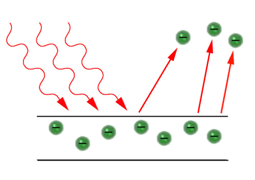
In the quantum description of the electromagnetic force, there is a particle which plays the role of the force carrier. That particle is called the photon. When the photon is a virtual particle, it mediates the force between charged particles. Real photons, though, are the particle version of the electromagnetic wave, meaning that a photon is a particle of light. It was Albert Einstein who realized particle-wave duality—his study of the photoelectric effect showed the particle nature of the electromagnetic field and won him the Nobel Prize.

Figure 12: When light shines on a metal, electrons pop out.

Here, we should make a distinction between what we mean by the electromagnetic field and the fields that fill the vacuum from the last section. The photon field is the one that characterizes the photon particle, and photons are vibrations in the photon field. However, charged particles—for instance, those in the nucleus of an atom—are surrounded by an electromagnetic field, which is in fact the photon field “turned on”. An analogy can be made with the string of a violin. An untouched string would be the dormant photon field. If one pulls the middle of the string without letting go, tension (and energy) is added to the string and the shape is distorted—this is what happens to the photon field around a stationary nucleus. And in that circumstance for historical reasons it is called the “electromagnetic field.” If the string is plucked, vibrations move up and down the string. If we jiggle the nucleus, an electromagnetic wave leaves the nucleus and travels the speed of light. That wave, a vibration of the photon field, can be called a “photon.”

So in general, there are dormant fields that carry all the information about the particles. Then, there are static fields, which are the dormant fields turned on but stationary. Finally, there are the vibrating fields (like the waves in the lake), which (by their quantum nature) can be described as particles.

The power of QED

The full quantum field theory describing charged particles and electromagnetic interactions is called quantum electrodynamics, or QED. In QED, charged particles, such as electrons, are fermions with half-integer spin that interact by exchanging photons, which are bosons with one unit of spin. Photons can be radiated from charged particles when they are accelerated, or excited atoms where the spin of the atom changes when the photon is emitted. Photons, with integer spin, are easily absorbed by or created from the photon field.

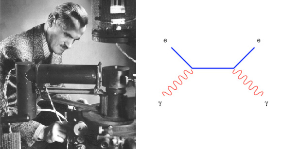
Figure 13: Arthur Holly Compton (left) discovered that the frequency of light can change as it scatters off of matter. Arthur Holly Compton (left), a physicist at Washington University in St. Louis, MO, did a careful measurement of light scattering off a crystal in 1923. He found that the frequency of light was related to the scattering angle: The frequency of scattered light decreased more when the light was scattered through larger angles. He explained this through the interaction of light (photons) with electrons in the crystal. On the right is a Feynman diagram representing a part of the calculation of Compton scattering. In the diagram, time increases to the right. An electron (blue) and a photon (red) interact in a way that can change the final energy and momentum of each particle. (Unit: 2)
Source: © Left: NASA, Right: David Kaplan.

QED describes the hydrogen atom beautifully. It also describes the high-energy scattering of charged particles. Physicists can accurately compute the familiar Rutherford scattering (see Unit 1) of a beam of electrons off the nuclei of gold atoms by using a single Feynman diagram to calculate the exchange of a virtual photon between the incoming electron and the nucleus. QED also gives, to good precision, the cross section for photons scattered off electrons. This Compton scattering has value in astrophysics as well as particle physics. It is important, for example, in computing the cosmic microwave background of the universe that we will meet in Unit 4. QED also correctly predicts that gamma rays, which are high-energy photons, can annihilate and produce an electron-positron pair when their total energy is greater than the mass energy of the electron and positron, as well as the reverse process in which an electron and positron annihilate into a pair of photons.

Physicists have tested QED to unprecedented accuracy, beyond any other theory of nature. The most impressive result to date is the calculation of the anomalous magnetic moment, a_μ, a parameter related to the magnetic field around a charged particle. Physicists have compared theoretical calculations and experimental tests that have taken several years to perform. Currently, the experimental and theoretical numbers for the muon are:

a_μ^exp = .0011659208±.0000000006

a_μ^th = .0011659183±.0000000006

These numbers reveal two remarkable facts: The sheer number of decimal places, and the remarkably close but not quite perfect match between them. The accuracy (compared to the uncorrected value of the magnetic moment) is akin to knowing the distance from New York to Los Angeles to within the width of a dime. While the mismatch is not significant enough to proclaim evidence that nature deviates from QED and the Standard Model, it gives at least a hint. More important, it reveals an avenue for exploring physics beyond the Standard Model. If a currently undiscovered heavy particle interacts with the muon, it could affect its anomalous magnetic moment and would thus contribute to the experimental value. However, the unknown particle would not be included in the calculated number, possibly explaining the discrepancy. If this discrepancy between the experimental measurement and QED calculation becomes more significant in the future, as more precise experiments are performed and more Feynman diagrams are included in the calculation, undiscovered heavy particles could make up the difference. The discrepancy would thus provide the starting point of speculation for new phenomena that physicists can seek in high-energy colliders.

Changing force in the virtual soup

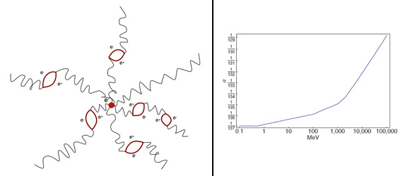
The strength of the electromagnetic field around an electron depends on the charge of the electron—a bigger charge means a stronger field. The charge is often called the coupling because it represents the strength of the interaction that couples the electron and the photon (or more generally, the matter particle and the force carrier). Due to the quantum nature of the fields, the coupling actually changes with distance. This is because virtual pairs of electrons and positrons are effectively popping in and out of the vacuum at a rapid rate, thus changing the perceived charge of that single electron depending on how close you are when measuring it. This effect can be precisely computed using Feynman diagrams. Doing so reveals that the charge or the electron-photon coupling grows (gets stronger) the closer you get to the electron. This fact, as we will see in the following section, has much more important implications about the theory of the strong force. In addition, it suggests how forces of different strength could have the same strength at very short distances, as we will see in the section on the unification of forces.

Figure 14: QED at high energies and short distances.The electromagnetic force, in its full quantum description, has the property that the coupling, or strength of charge, is different when it is measured at different energies. Probing an electron at high energy is equivalent to probing it at short range. The electromagnetic field around the electron has quantum fluctuations that include the appearance of virtual pairs of electrons and positrons as shown on the left. Those virtual effects change the perceived coupling as one gets closer or farther from the electron. The plot on the right gives the measured strength of the coupling, at different scattering energies (given in MeV). (Unit: 2) Source: © David Kaplan.

The other force, in addition to the electromagnetic force, that plays a significant role in the structure of the atom is the strong nuclear force. Like the electromagnetic force, the strong force can create bound states that contain several particles. Their bound states, such as nuclei, are around 10^-15 meters in diameter, much smaller than atoms, which are around 10^-10 meters across. It is the energy stored in the bound nuclei that is released in nuclear fission, the reaction that takes place in nuclear power plants and nuclear weapons, and nuclear fusion, which occurs in the center of our Sun and of other stars.

Confined quarks

We can define charge as the property particles can have that allow them to interact via a particular force. The electromagnetic force, for example, occurs between particles that carry electric charge. The value of a particle’s electric charge determines the details of how it will interact with other electrically charged particles. For example, electrons have one unit of negative electric charge. They feel electromagnetic forces when they are near positively charged protons, but not when they are near electrically neutral neutrinos, which have an electric charge of zero. Opposite charges attract, so the electromagnetic forces tends to create electrically neutral objects: Protons and electrons come together and make atoms, where the positive and negative charges cancel. Neutral atoms can still combine into molecules, and larger objects, as the charged parts of the atoms attract each other.

Figure 15: Neutralized charges in QED and QCD.
Source: © David Kaplan.

At the fundamental particle level, it is quarks that feel the strong force. This is because quarks have the kind of charge that allows the strong force to act on them. For the strong force, there are three types of positive charge and three types of negative charge. The three types of charge are labeled as colors —a quark can come in red, green, or blue. Antiquarks have negative charge, labeled as anti-red, etc. Quarks of three different colors will attract each other and form a color-neutral unit, as will a quark of a given color and an antiquark of the same anti-color. As with the atom and the electromagnetic force, baryons such as protons and neutrons are color-neutral (red+green+blue=white), as are mesons made of quarks and antiquarks, such as pions. Protons and neutrons can still bind and form atomic nuclei, again, in analogy to the electromagnetic force binding atoms into molecules. Electrons and other leptons do not carry color charge and therefore do not feel the strong force.

In analogy to quantum electrodynamics, the theory of the strong force is called quantum chromodynamics, or QCD. The force carrier of the strong force is the gluon, analogous to the photon of electromagnetism. A crucial difference, however, is that while the photon itself does not carry electromagnetic charge, the gluon does carry color charge—when a quark emits a gluon, that actually changes its color. Because of this, the strong force binds particles together much more tightly. Unlike the electromagnetic force, whose strength decreases as the inverse square distance between two charged particles (that is, as 1/r², where r is the distance between particles), the strong force between a quark and antiquark remains constant as the distance between them grows.

Figure 16: As two bound quarks are pulled apart, new quarks pop out of the vacuum. The strong force is strong because when particles with color charge are pulled apart, the force strength does not diminish, as it does in QED. The force field is said to form a string or tube between a quark and anti-quark being pulled apart. When the string gets long enough, it contains more energy than it takes to create new particles by converting that energy into mass. In that case, a quark and anti-quark pair can appear out of the vacuum, canceling the color charge of each of the other two, and breaking the string.
Source: © David Kaplan.

The gluon field is confined to a tube that extends from the quark to the antiquark because, in a sense, the exchanged gluons themselves are attracted to each other. These gluon tubes have often been called strings. In fact, the birth of string theory came from an attempt to describe the strong interactions. It has moved on to bigger and better things, becoming the leading candidate for the theory of quantum gravity as we’ll see in Unit 4.

As we pull bound quarks apart, the gluon tube cannot grow indefinitely. That is because it contains energy. Once the energy in the tube is greater than the energy required to create a new quark and antiquark, the pair pops out of the vacuum and cuts the tube into two smaller, less energetic, pieces. This fact—that quarks pop out of the vacuum to form new hadrons—has dramatic implications for collider experiments, and explains why we do not find single quarks in nature.

Particle jets

Particle collisions involving QCD can look very different than those involving QED. When a proton and an antiproton collide, one can imagine it as two globs of jelly hurling toward each other. Each glob has a few marbles embedded in them. When they collide, once in a while two marbles find each other, make a hard collision, and go flying out in some random direction with a trail of jelly following. The marbles represent quarks and gluons, and in the collision, they are being torn from the jelly that is the proton.

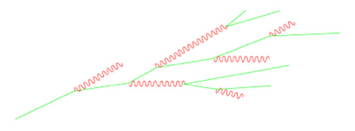
Figure 17: In this Feynman diagram of a jet, a single quark decays into a shower of quarks and gluons. When quarks and anti-quarks and gluons are produced in high-energy collisions, they move apart from each other at nearly the speed of light. The immediate response is to start pulling more color-charged particles out of the vacuum, mostly in the direction the original particle is moving. Thus, the signature of a high-energy quark or gluon produced in a particle collider is a spray of hadrons, most confined to a small cone, or jet, whose vertex is at the collision point. In the diagram above, quarks are represented by straight green lines and gluons are red wiggly lines. Time increases to the right. (Unit: 2)
Source: © David Kaplan.

However, we know quarks cannot be free, and that if quarks are produced or separated in a high-energy collision, the color force starts ripping quark/anti-quark pairs out of the vacuum. The result is a directed spray, or jet of particles headed off in the direction the individual quark would have gone. This can be partially described by a Feynman diagram where, for example, a quark becomes a shower of quarks and gluons.

In the early days of QCD, it became clear that if a gluon is produced with high energy after a collision, it, too, would form a jet. At that point, experimentalists began to look for physical evidence of gluons. In 1979, a team at the newly built PETRA electron-positron storage ring at DESY, Germany’s Deutsches Elektronen-Synchrotron, found the evidence, in the form of several of the tell-tale three-jet events. Other groups quickly confirmed the result, and thus established the reality of the gluon.

A confining force

As we have seen, the strength of the strong force changes depending on the energy of the interaction, or the distance between particles. At high energies, or short distances, the strong force actually gets weaker. This was discovered by physicists David Gross, David Politzer, and Frank Wilczek, who received the 2004 Nobel Prize for this work. In fact, the color charge (or coupling) gets so weak at high energies, you can describe the interactions between quarks in colliding protons as the scattering of free quarks; marbles in jelly are a good metaphor.

Figure 18: The QCD coupling depends on energy. Just like in QED, the coupling of the strong force changes its measured value as one gets closer or farther from a quark. This is again due to the effect of virtual particles in the field. The difference, due to the fact that the gluons carry color and anti-color, is that the QCD coupling strength gets smaller as one probes it closer. This effect, called asymptotic freedom, means that the higher in energy you go, the weaker the force gets, up to a point where in the scattering, the quarks act as if they are free instead of bound. (Unit: 2)

At lower energies, or longer distances, the charge strength appears to hit infinity, or blows up as physicists like to say. As a result, protons may as well be a fundamental particle in low-energy proton-proton collisions because the collision energy isn’t high enough to probe their internal structure. In this case, we say that the quarks are confined. This qualitative result is clear in experiments, however, “infinity” doesn’t make for good quantitative predictions. This difficulty keeps QCD a lively and active area of research.

Physicists have not been able to use QCD theory to make accurate calculations of the masses and interactions of the hadrons made of quarks. Theorists have developed a number of techniques to overcome this issue, the most robust being lattice gauge theory. This takes a theory like QCD, and puts it on a lattice, or grid of points, making space and time discrete rather than continuous. And because the number of points is finite, the situation can be simulated on a computer. Amazingly enough, physicists studying phenomena at length scales much longer than the defined lattice point spacing find that the simulated physics acts as if it is in continuous space. So, in theory, all one needs to do to calculate the mass of a hadron is to space the lattice points close enough together. The problem is that the computing power required for a calculation grows exponentially with the number of points on the lattice. One of the main hurdles to overcome in lattice gauge theory at this point is the computer power needed for accurate calculations.

The pion puzzle

The energy scale where the QCD coupling blows up is in fact the mass of most hadrons—roughly 1 GeV. There are a few exceptions, however. Notably, pions are only about a seventh the mass of the proton. These particles turn out to be a result of spontaneous symmetry breaking in QCD as predicted by the so-called Nambu-Goldstone theorem that we will learn more about in Section 8.

Japanese physicist Hideki Yukawa predicted the existence of the pion, a light spinless particle, in 1935. Yukawa actually thought of the pion as a force carrier of the strong force, long before QCD and the weak forces were understood, and even before the full development of QED. Yukawa believed that the pion mediated the force that held protons and neutrons together in the nucleus. We now know that pion exchange is an important part of the description of low-energy scattering of protons and neutrons.

Yukawa’s prediction came from using the Heisenberg uncertainty principle in a manner similar to what we did in Section 2 when we wanted to understand the exchange of force carriers. Heisenberg’s uncertainty principle suggests that a virtual particle of a certain energy (or mass) tends to exist for an amount of time (and therefore tends to travel a certain distance) that is proportional to the inverse of its energy. Yukawa took the estimated distance between protons and neutrons in the nucleus and converted it into an energy, or a mass scale, and predicted the existence of a boson of that mass. This idea of a heavy exchange particle causing the force to only work at short distances becomes the central feature in the next section.

Neither the strong force nor the electromagnetic force can explain the fact that a neutron can decay into a proton, electron, and an (invisible) antineutrino. For example carbon–14, an atom of carbon that has six protons and eight neutrons, decays to nitrogen–14 by switching a neutron to a proton and emitting an electron and antineutrino. Such a radioactive decay (called beta decay) led Wolfgang Pauli to postulate the neutrino in 1930 and Enrico Fermi to develop a working predictive theory of the particle three years later, leading eventually to its discovery by Clyde Cowan, Jr. and Frederick Reines in 1956. For our purposes here, what is important is that this decay is mediated by a new force carrier—that of the weak force.

Figure 19: An example of beta decay. In this example of beta-minus decay, carbon-14 decays to nitrogen-14, an electron and an anti-neutrino. We can interpret this as a neutron changing into a proton and emitting the electron and anti-neutrino. While this is a decay, and not an interaction, it is mediated by the weak force—the only force that changes particle type. (Unit: 2)

As with QED and QCD, the weak force carriers are bosons that can be emitted and absorbed by matter particles. They are the electrically charged W⁺ and W^–, and the electrically neutral Z⁰. There are many properties that distinguish the weak force from the electromagnetic and strong forces, not the least of which is the fact that it is the only force that can mediate the decay of fundamental particles. Like the strong force, the theory of the weak force first appeared in the 1930s as a very different theory.

Fermi theory and heavy force carriers

SETTING THE STAGE FOR UNIFICATION

Chen-Ning Yang and Robert Mills created a mathematical construct that lay the groundwork for future efforts to unify the forces of nature.
© picture taken by A.C.T. Wu (Univ. of Michigan) at the 1999 Yang Retirement Symposium at Stony Brook, Courtesy of AIP, Emilio Segrè Visual Archives.

When they shared an office at the Brookhaven National Laboratory in 1954, Chen-Ning Yang and Robert Mills created a mathematical construct that lay the groundwork for future efforts to unify the forces of nature. The Yang-Mills theory generalized QED to have more complicated force carriers—ones that interact with each other—in a purely theoretical construct. The physics community originally showed little enthusiasm for the theory. But in the 1960s and beyond the theory proved invaluable to physicists who eventually won Nobel Prizes for their work in uniting electromagnetism and the weak force and understanding the strong force. Yang himself eventually won a Nobel Prize with T.D. Lee for the correct prediction of (what was to become) the weak-force violation of parity invariance. Yang’s accomplishments place him as one of the greatest theoretical physicists of the second half of the 20th century.

Fermi constructed his theory of beta decay in 1933, which involved a direct interaction between the proton, neutron, electron,and antineutrino (quarks were decades away from being postulated at that point). Fermi’s theory could be extended to other particles as well, and successfully describes the decay of the muon to an electron and neutrinos with high accuracy. However, while the strength of QED (its coupling) was a pure number, the strength of the Fermi interaction depended on a coupling that had the units of one over energy squared. The value of the Fermi coupling (often labeled G_F) thus suggested a new mass/energy scale in nature associated with its experimental value: roughly 250 times the proton mass (or ~250 GeV).

In 1961, a young Sheldon Glashow fresh out of graduate school, motivated by experimental data at the time, and inspired by his advisor Julian Schwinger’s work on Yang-Mills theory, proposed a set of force carriers for the weak interactions. They were the W and Z bosons, and had the masses necessary to reproduce the success of Fermi theory. The massive force carriers are a distinguishing feature of the weak force when compared with the massless photon and essentially massless (yet confined) gluon. Thus, when matter is interacting via the weak force at low energies, the virtual W and Z can only exist for a very short time due to the uncertainty principle, making the weak interactions an extremely short-ranged force.

Another consequence of heavy force carriers is the fact that it requires a large amount of energy to produce them. The energy scale required is associated with their mass (M_wc²) and is often called the weak scale. Thus, it was only in the early 1980s, nearly a century after seeing the carriers’ effects in the form of radioactivity, that scientists finally discovered the W and Z particles at the UA1 experiment at CERN.

Figure 20: Neutron decay from the inside.
When a neutron decays, one of its constituent down quarks changes into an up quark by emitting a virtual weak force carrier, the W boson. The change happens deep within the hadron, as the W lasts only a very short time, before the neutron “knows” what happened. (Unit: 2)
Source: © David Kaplan

Force of change

An equally important difference between the weak force and the others is that when some of the force carriers are emitted or absorbed (specifically, the W^+/-), the particle doing the emitting/absorbing changes its flavor. For example, if an up quark emits a W⁺, it changes into a down quark. By contrast, the electron stays an electron after it emits or absorbs QED’s photon. And while the gluon of QCD changes the color of the quark from which it is emitted, the underlying symmetry of QCD makes quarks of different colors indistinguishable. The weak force does not possess such a symmetry because its force carrier, the W, changes one fermion into a distinctly different one. In our example above, the up and down quarks have different masses and electric charges. However, physicists have ample theoretical and indirect experimental evidence that the underlying theory has a true symmetry. But that symmetry is dynamically broken because of the properties of the vacuum, as we shall see later on.

That fact that the W boson changes the flavor of the matter particle has an important physical implication: The weak force is not only responsible for interactions between particles, but it also allows heavy particles to decay. Because the weak force is the only one that changes quarks’ flavors, many decays in the Standard Model, such as that of the heavy top quark, could not happen without it. In its absence, all six quark flavors would be stable, as would the muon and the tau particles. In such a universe, stable matter would consist of a much larger array of fundamental particles, rather than the three (up and down quarks and the electron) that make up matter in our universe. In such a universe, it would have taken much less energy to discover the three generations, as we would simply detect them. As it is, we need enough energy to produce them, and even then they decay rapidly and we only get to see their byproducts.

Weak charge?

In the case of QED and QCD, the particles carried the associated charges that could emit or absorb the force carriers. QED has one kind of charge (plus its opposite, or conjugate charge), which is carried by all fundamental particles except neutrinos. In QCD, there are three kinds of color charge (and their conjugates) which are only carried by quarks. Therefore, only quarks exchange gluons. In the case of the weak force, all matter particles interact with and thus can exchange the W and Z particles—but then what exactly is weak charge?

Figure 21: The total amount of electric charge is conserved, even in complicated interactions like this one. Electromagnetic charge is conserved. This means the total charge of a system (number of positive minus number of negative charges) remains the same, no matter what physical process occurs. In the interaction shown here, the net electromagnetic charge of the system is -2 throughout the interaction. This is not true of the weak force charge. (Unit: 2)
Source: © David Kaplan.

An important characteristic feature of electromagnetic charge is that it is conserved. This means, for any physical process, the total amount of positive charge minus the total amount of negative charge in any system never changes, assuming no charge enters or leaves the system. Thus, positive and negative charge can annihilate each other, or be created in pairs, but a positive charge alone can never be destroyed. Similarly for the strong force, the total amount of color charge minus the total anti-color charge typically stays the same, there is one subtlety. In principle, color charge can also be annihilated in threes, except for the fact that baryon number—the number of baryons like protons and neutrons—is almost exactly conserved as well. This makes color disappearance so rare that it has never been seen.

Weak charge, in this way, does not exist—there is no conserved quantity associated with the weak force like there is for the other two. There is a tight connection between conserved quantities and symmetries. Thus, the fact that there is no conserved charge for the weak force is again suggestive of a broken symmetry.

Look in the mirror—it’s not us

Figure 22: For the weak force, an electron’s mirror image is a different type of object. KaplanThe electron on the left has an effective rotation that is counter-clockwise when looked at along the direction of motion (i.e., from behind). The mirror image is an electron rotating clockwise when seen along the direction of motion. Physicists call the former left-handed and the latter right-handed. Because the weak force treats the left-handed electron and right-handed electron differently, the world inside the mirror has different interactions than our world! (Unit: 2)  Source: © David Kaplan

The weak interactions violate two more symmetries that the strong and electromagnetic forces preserve. As discussed in the previous unit, these are parity(P) and charge conjugation (C). The more striking one is parity. A theory with a parity symmetry is one in which any process or interaction that occurs (say particles scattering off each other, or a particle decaying), its exact mirror image also occurs with the same probability. One might think that such a symmetry must obviously exist in Nature. However, it turns out that the weak interactions maximally violate this symmetry.

As a physical example, if the W^– particle is produced at rest, it will—with roughly 10% probability—decay into an electron and an antineutrino. What is remarkable about this decay is that the electron that comes out is almost always left-handed. A left-handed (right-handed) particle is one in which when viewed along the direction it is moving, its spin is in the counterclockwise (clockwise) direction. It is this fact that violates parity symmetry, as the mirror image of a left-handed particle is a right-handed particle.

Figure 23: Spin flipping on the train. A left-handed electron is seen from a stopped train (left). If the train starts moving faster than the electron, it will appear to be moving the other way, and thus will appear right-handed. If the electron had zero mass, it would move at the speed of light, and thus no train would be able to overtake it. In that case, the left-handed and right-handed electrons would be truly distinct particles. (Unit: 2) Source: © David Kaplan

The electron mass is very tiny compared to that of the W boson. It turns out that the ability of the W^– to decay into a right-handed electron depends on the electron having a mass. If the mass of the electron were zero in the Standard Model, the W^– would only decay into left-handed electrons. It is the mass, in fact, that connects the left-handed and right-handed electrons as two parts of the same particle. To see why, imagine an electron moving with a left-handed spin. If you were to travel in the same direction as the electron, but faster, then the electron to you would look as if it were moving in the other direction, but its spin would be in the original direction. Thus, you would now see a right-handed electron. However, if the electron had no mass, Einstein’s relativity would predict that it moves at the speed of light (like the photon), and you would never be able to catch up to it. Thus, the left-handed massless electron would always look left-handed.

The mixing of the left- and right-handed electrons (and other particles) is again a result of a symmetry breaking. The symmetry is sometimes called chiral symmetry, from the Greek word chiral, meaning hand. The masses of the force carriers, the flavor-changing nature of the weak force, and the masses of all matter particles, all have a single origin in the Standard Model of particle physics—the Higgs mechanism—as we will see in the next section.

While the W particles are force carriers of the weak force, they themselves carry charges under the electromagnetic force. While it is not so strange that force carriers are themselves charged—gluons carry color charges, for example—the fact that it is electromagnetic charge suggests that QED and the weak force are connected. Glashow’s theory of the weak force took this into account by allowing for a mixing between the weak force and the electromagnetic force. The amount of mixing is labeled by a measurable parameter, θ_w.

Unifying forces

The full theory of electroweak forces includes four force carriers: W⁺, W^–, and two uncharged particles that mix at low energies—that is, they evolve into each other as they travel. This mixing is analogous to the mixing of neutrinos with one another discussed in the previous unit. One mixture is the massless photon, while the other combination is the Z. So at high energies, when all particles move at nearly the speed of light (and masses can be ignored), QED and the weak interactions unify into a single theory that we call the electroweak theory. A theory with four massless force carriers has a symmetry that is broken in a theory where three of them have masses. In fact, the Ws and Z have different masses. Glashow put these masses into the theory by hand, but did not explain their origin.

This is a display of tracks of particles emanating from a Z particle produced at the Stanford Linear Collider (SLAC). This picture is viewed “head-on” along the beam line. The collider produced more than half a million Z particles during its seven years of operation, while the Large Electron-Positron collider (LEP), running at the same time, produced over 17 million. (Unit: 2)
Source: © SLAC National Accelerator Laboratory

The single mixing parameter predicts many different observable phenomena in the weak interactions. First, it gives the ratio of the W and Z masses (it is the cosine of ). It also gives the ratio of the coupling strength of the electromagnetic and weak forces (the sine of ). In addition, many other measurable quantities, such as how often electrons or muons or quarks are spinning one way versus another when they come from a decaying Z particle, depend on the single mixing parameter. Thus, the way to test this theory is to measure all of these things and see if you get the same number for the one parameter.

Testing of the electroweak theory has been an integral part of particle physics experimental research from the late 1980s until today. For example, teams at LEP (the Large Electron-Positron collider, which preceded the Large Hadron Collider (LHC) at CERN) produced 17 million Z bosons and watched them decay in different ways, thus measuring their properties very precisely, and putting limits on possible theories beyond the Standard Model. The measurements have been so precise that they needed an intensive program on the theoretical side to calculate the small quantum effects (loop diagrams) so theory and experiment could be compared at similar accuracy.

A sickness and a cure

While the electroweak theory could successfully account for what was observed experimentally at the time of its inception, one could imagine an experiment that could not be explained. If one takes this theory and tries to compute what happens when Standard Model particles scatter at very high energies (above 1 TeV) using Feynman diagrams, one gets nonsense. Nonsense looks like, for example, probabilities greater than 100%, measurable quantities predicted to be infinity, or simply approximations where the next correction to a calculation is always bigger than the last. If a theory produces nonsense when trying to predict a physical result, it is the wrong theory.

A “fix” to a theory can be as simple as a single new field (and therefore, particle). We need a particle to help Glashow’s theory, so we’ll call it H. If a particle like H exists, and it interacts with the known particles, then it must be included in the Feynman diagrams we use to calculate things like scattering cross sections. Thus, though we may never have seen such a particle, its virtual effects change the results of the calculations. Introducing H in the right way changes the results of the scattering calculation and gives sensible results.

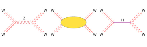
Figure 25: Scattering of W particles in Feynman diagrams. The three Feynman diagrams above represent parts of the calculation of the probability of two W particles scattering. The first, and others like it, together represent the calculation including all known particles. When calculated for very high energy W particles, the result is nonsense. The way out is if there are unknown diagrams which, when included, yield sensible answers. The yellow blob in the middle picture represents the unknown part of the diagram. It turns out that simplest way to make sense of this calculation is to add a single new particle—the Higgs boson—and include all possible new diagrams, including the one on the right. (Unit: 2) Source: © David Kaplan

In the mid-1960s, a number of physicists, including Scottish physicist Peter Higgs, wrote down theories in which a force carrier could get a mass due to the existence of a new field. In 1967, Steven Weinberg (and independently, Abdus Salam), incorporated this effect into Glashow’s electroweak theory producing a consistent, unified electroweak theory. It included a new particle, dubbed the Higgs boson, which, when included in the scattering calculations, completed a new theory—the Standard Model—which made sensible predictions even for very high-energy scattering.

A mechanism for mass

The way the Higgs field gives masses to the W and Z particles, and all other fundamental particles of the Standard Model (the Higgs mechanism), is subtle. The Higgs field—which like all fields lives everywhere in space—is in a different phase than other fields in the Standard Model. Because the Higgs field interacts with nearly all other particles, and the Higgs field affects the vacuum, the space (vacuum) particles travel through affects them in a dramatic way: It gives them mass. The bigger the coupling between a particle and the Higgs, the bigger the effect, and thus the bigger the particle’s mass.

In our earlier description of field theory, we used the analogy of waves traveling across a lake to represent particles moving through the vacuum. A stone thrown into a still lake will send ripples across the surface of the water. We can imagine those ripples as a traveling packet of energy that behaves like a particle when it is detected on the other end. Now, imagine the temperature drops and the lake freezes; waves can still exist on the surface of the ice, but they move at a completely different speed. So, while it is the same lake made of the same material (namely, water), the waves have very different properties. Things attempting to move through the lake (like fish) will have a very different experience trying to get through the lake. The change in the state of the lake itself is called a phase transition.

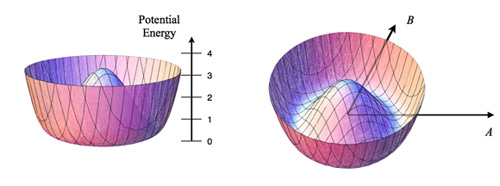
Figure 26: The Higgs mechanism is analogous to a pond freezing over. The Higgs mechanism is described by a field filling all space that goes through something like a phase change and gives mass to itself and most particles of the Standard Model. The movie above is a (very) loose analogy. The lake represents the field, and a particle could be the ripples moving across the surface. If the lake freezes (changes from the liquid phase to the solid phase), the slow moving ripples no longer occur. The ice can instead vibrate. Thus, the character of the waves has completely changed when the material changes its phase. It is the “condensation” of the Higgs field that changed (in the early universe) the character of the fundamental particles we see.
Source: © David Kaplan.

This situation with the Higgs has a direct analogy with the freezing lake. At high enough temperatures, the Higgs field does not condense, which means that it takes on a constant value everywhere, and the W and Z are effectively massless. Lower temperatures can cause a transition in which the Higgs doublet condenses, the W and Z gain mass, and it becomes more difficult for them to move through the vacuum, as it is for fish in the lake, or boats on the surface when the lake freezes. In becoming massive, the W and Z absorb parts of the Higgs field. The remaining Higgs field has quantized vibrations that we call the Higgs boson that are analogous to vibrations on the lake itself. This effect bears close analogy with the theory of superconductivity that we will meet in Unit 8. In a sense, the photon in that theory picks up a mass in the superconducting material.

Not only do the weak force carriers pick up a mass in the Higgs phase, so do the fundamental fermions—quarks and leptons—of the Standard Model. Even the tiny neutrino masses require the Higgs effect in order to exist. That explains why physicists sometimes claim that the Higgs boson is the origin of mass. However, the vast majority of mass in our world comes from the mass of the proton and neutron, and thus comes from the confinement of the strong interactions. On the other hand, the Higgs mechanism is responsible for the electron’s mass, which keeps it from moving at the speed of light and therefore allows atoms to exist. Thus, we can say that the Higgs is the origin of structure.

Closing in on the Higgs

There is one important parameter in the electroweak theory that has yet to be measured, and that is the mass of the Higgs boson. Throughout the 1990s and onward, a major goal of the experimental particle physics community has been to discover the Higgs boson. The LEP experiments searched for the Higgs to no avail and have put a lower limit on its mass of 114 Giga-electron-volts (GeV), or roughly 120 times the mass of the proton. For the Standard Model not to produce nonsense, the Higgs must appear in the theory at energies (and therefore at a mass) below 1,000 GeV.

Figure 27: Simulation of a Higgs event at the LHC. This is the simulation of a display of LHC detector information in the event of a Higgs being produced. Careful measurement of the energy and other properties of the tracks of the outgoing particles will allow experimentalists to reconstruct what might have happened at the collision point. Any one “Higgs event” could be a random accident, while collections of millions of these types of events, along with careful analysis, can give physicists confidence they are seeing something new. (Unit: 2) Source: © ATLAS Experiment, CERN.

However, there have been stronger, more indirect ways to narrow in on the Higgs. When LEP and other experiments were testing the electroweak theory by making various measurements of the mixing angle, the theory calculations needed to be very precise, and that required the computing of more complicated Feynman diagrams. Some of these diagrams included a virtual Higgs particle, and thus the results of these calculations depend on the existence of the Higgs.

Though the effects of virtual Higgs bosons in Feynman diagrams are subtle, the experimental data is precise enough to be sensitive to the mass to the Higgs. Thus, though never seen, as of 2010, there is a prediction that the Higgs boson mass must be less than roughly 200 times the proton mass. With a successful high-energy run of the Large Hadron Collider, and with the support of a full analysis of data from the Tevatron experiments at Fermilab, we should know a lot about the Higgs boson, whether it exists, and what its mass is by 2015.

Symmetries are a central tool in theoretical physics. They can play the role of an organizing principle in a new theory, or can allow for tremendous simplification of otherwise difficult problems. In particle physics, theorists speculate about new symmetry principles when they seek deeper explanations or theories of fundamental particles or forces. Condensed matter physicists use symmetries to characterize the molecular structure of different materials. Atomic physicists organize atomic states in terms of rotational symmetry. Without symmetries—even approximate symmetries—it is extremely difficult to characterize the properties of physical systems.

Exact and approximate symmetries in particle physics

A system has a symmetry when changing the system in some way leaves it in an identical state. For example, a perfect circle, when rotated around the center, looks the same. We call rotating the circle—or any change of the system that leaves it looking the same—a symmetry transformation. The set of all symmetry transformations—all things that can be done to the system and leave it looking the same—form a group, a word with a precise mathematical definition. The transformations can be continuous, as a rotation by an arbitrary angle, or discrete, as a flip to a mirror image.

Figure 28: Rotations in physical space and “particle space.” Rotations in physical space are analogous to rotations in “particle space.” One can represent the changing of a particle from one type to another as a rotating arrow. The picture above shows an arrow that is rotated from an eastward direction to something between east and north. The picture on the right shows an arrow which is rotated from the A direction to something between A and B. The direction represents what the particle type is, and thus allows a description in which the particle is neither A nor B, but a combination of the two. If the theory has a symmetry with respect to particle type, it means that physics experiments do not depend on which direction the arrow is pointing—which particle, or particle combination, is in the experiment. (Unit: 2)
Source: © David Kaplan.

Symmetries can apply not only to external properties, like physical rotations, but also to internal properties, like particle type. For example, a symmetry could exist where all physics experiments done with particle A would yield the same results with the same probabilities if they were done with particle B. This implies an exchange symmetry between A and B: You get the same result if you exchange particle A for particle B, and vice versa. In this case, the two particles have precisely the same properties.

More general and stranger symmetries can exist as well. For example, instead of simply exchanging particles A and B, one could replace particle A with a particle that is partially A and partially B. This occurs in the case of neutrinos, where one flavor is produced—for example, electron neutrinos in the sun—and another is measured far away—muon or tau neutrinos on earth. It is also true in the case of uncharged mesons made of quarks, like neutral Kaons or B-mesons. Thus, this kind of symmetry of A and B could be described as a “rotation” between particle types—it could be one or the other or a mixture of the two. It is very similar to physical direction, in the sense that one could be facing north or east or in some mixture of the two (e.g., east-north-east).

If one wanted to do a measurement to tell whether a particle is A or B, there would have to be something to distinguish the two—some difference. But a difference would mean the symmetry is not exact. One example is the three neutrinos of the Standard Model. They are almost, but not quite, the same. The distinction is that electron neutrinos interact in a special way with electrons, whereas muon and tau neutrinos interact in that same way with muon and tau particles, respectively. So here, the symmetry is approximate because the particles the neutrinos are associated with have very different masses. Exchanging a neutrino of one species with another changes how it interacts with the electron, for example. Also, when a neutrino scatters off of matter, the matter can ‘pick out’ the flavor of neutrino and change it to one type or another.

Figure 29: A combination particle that’s a mixture of type A and type B can be turned into a pure type A or pure type B particle when it interacts with matter. A particle that is some combination of type A and type B comes in and scatters off of a target. The target knows the difference between A and B, and when the particle scatters, it becomes an A particle alone. An example of this is the neutrino, which can be a mixture of different types, but will scatter off of matter in a certain way only if it is an electron type neutrino. The neutrino might start off as a combination of electron, muon, and tau flavors. By scattering, the neutrino becomes a pure electron neutrino.
Source: © David Kaplan.

What if the three neutrinos of the Standard Model were exactly the same—how would we ever know that there are three? It turns out that we can determine the number of light neutrinos from experimental measurements of Z bosons. The decay rate of the Z boson depends on how many light particles are coupled to it and the size of their couplings. Since the couplings can be measured in other ways, and the decays of the Z that don’t involve neutrinos are visible, i.e., they leave energy in the detector, one can infer the number of neutrinos. The number measured in this way is ~2.984, in agreement (within errors) with the three neutrinos of the Standard Model.

Spontaneous symmetry breaking

It might seem as though a system either has a symmetry or it doesn’t: We can rotate a circle by any angle and it looks the same, but that doesn’t work for a square. However, it is possible for a physical theory to have a symmetry that isn’t reflected in the current state of the system it describes. This can happen when a symmetry is spontaneously broken.

What does that mean? Consider, for example, a spinning top, whose point remains stationary on a table. The system (the top) is perfectly symmetric around its spinning axis—looking at the top from any side of the table, one sees the same image. Once the top has finished spinning, it lies on the table. The symmetry is gone, and the top no longer looks the same when viewed from any angle around the table. The top’s handle now points in a specific direction, and we see different things from different vantage points. However, the top could have fallen in any direction—in fact, one could say that the top has equal probability of pointing in any direction. Thus, the symmetry is inherent in the theory of the top, while that state of the system breaks the symmetry because the top has fallen in a particular direction. The symmetry was spontaneously broken because the top just fell over naturally as its rotational speed decreased.

Figure 30: The wine-bottle potential that is characteristic of spontaneous symmetry breaking. This shape represents the energy of the fields A and B for every possible value of A and B. If the fields both have zero value, the energy is represented by the top of the central hump. Physical systems tend to evolve towards their lowest energy state, so the values of the fields want to be greater than zero—i.e., they want to roll down the hill. The lowest energy the fields can have is at the bottom of the ring. The energy anywhere around the ring is the same, but A and B take on different values. One example of this is when the A field has a non-zero value (of the ring’s radius) and the B field is zero. That represents the point on the ring which is on the A arrow in the right-hand diagram. (Unit: 2)
Source: © David Kaplan.

One can have a similar spontaneous breaking of an internal symmetry. Imagine two fields, A and B, whose potential energies depend on each other in the way illustrated in Figure 30. While typically in theories, the lowest energy value of a field is zero, here we see the minimum energy value lies along the circular ring at the bottom. While the potential energy shape is symmetric—it looks the same rotated around the center—the fields take a particular value along the minimum-energy ring at every point in space, thus breaking the symmetry.

In Section 2, we learned that particles are simply fluctuations of a field. Our fields A and B can fluctuate in a very special way because the potential energy minimum forms a ring. If the fields are valued such that they sit in that minimum, and they fluctuate only around the ring, the potential energy does not change as the field fluctuates. Because the field vibrations involve no potential energy, the waves of the field can be as long and as low-energy as one wishes. Thus, they correspond to one or more massless particles. The fact that spontaneously breaking a symmetry results in a massless particle is known as the Nambu-Goldstone theorem, after physicists Yoichiro Nambu and Jeffrey Goldstone.

Figure 31: A wave in field space corresponds to a physical particle. This movie represents an A-B potential (from the previous figure), looking from the top, at every point in space. The black crosses represent the A and B directions, and the red lines start off pointing in the A direction. A wave—a packet of energy that we could also interpret as a particle—is shown as a coherent wiggling of the red line from the A position to somewhere between A and B. Because it doesn’t cost potential energy for the arrow to point in different directions, the wave can be as long and gentle as one likes. In particle language, this corresponds to a particle with no mass-energy, or no mass.
Source: © David Kaplan.

Pions, originally thought to be carriers of the strong force, are a real-life example of Nambu-Goldstone bosons. They are associated with the breaking of a complicated symmetry that involves the change of left-handed quarks into each other, with a simultaneous opposite change to right-handed quarks. This symmetry is spontaneously broken by the dynamics of the strong force in, as of today’s knowledge, some inexplicable way. Pions are light, rather than massless, because the symmetry is approximate rather than exact. Knowing that the pions are Nambu-Goldstone bosons allows physicists to determine some of the mysteries of how the strong force actually works.

Recovering symmetry at high temperatures

In our initial example of the spinning top, the theory had an underlying symmetry that was broken when the top fell over. When the top had a lot of energy and was spinning quickly, the symmetry was obvious. It was only when the top lost enough energy that it fell over that the symmetry was broken. The high-energy top displays a symmetry that the low-energy top does not. Something similar happens in more complicated systems such as magnets, superconductors, and even the universe.

Let’s take a magnet as an example. Make it a ball of iron to keep things nice and symmetric. The magnetization of iron comes about because the electrons, which are themselves tiny magnets, tend to want to line up their spine, and thus their magnetic fields, such that collectively, the entire material is magnetic. If one dumps energy in the form of heat into the magnet, the electrons effectively vibrate and twist more and more violently until at a critical temperature, 768 degrees Celsius for iron, the directions of their individual spins are totally randomized. At that point, the magnetic field from all of the electrons averages out to zero, and the iron ball is no longer magnetic.

When the iron is magnetized it is like the fallen top, having selected a particular direction as different from the rest. Once heated to the critical temperature, however, symmetry is restored and any direction within the magnet is equivalent to any other. Many symmetries that are spontaneously broken in the minimum energy state are restored at high temperatures. The Higgs mechanism we encountered in the previous section is a significant, if complicated, example. The restoration of symmetry at high temperatures has significant implications for the early universe, when the temperatures were extremely hot—it implies that at times very soon after the Big Bang, most or all of the spontaneously broken symmetries of the Standard Model (and its underlying theory) were intact.

The electromagnetic, strong, and weak interactions fit nicely into the Standard Model, and unify into a single theory at high temperatures. Gravity is still an outlier, in more ways than one. It is the first force to have a quantitative model thanks to Isaac Newton, and it happens to be the weakest force at the particle level. The electric force that binds a proton and electron into an atom is 10,000,000,000,000,000,000,000,000,000,000,000,000,000 (10⁴⁰) times larger than the gravitational force that attracts them.

Despite its weakness, gravity has a significant impact at macroscopic distances because of one crucial unique feature: All matter has the same sign gravitational charge. The charge for the gravitational force is mass, or energy in the full theory of general relativity. The gravitational force between two massive particles is always positive and it always attracts. Thus, unlike say electromagnetism, in which opposite charges attract and can thus screen the long-distant effects, gravitational charge always adds, and large objects can produce large gravitational fields.

Figure 32: Schematic of a laser interferometer that can detect gravitational waves. Physicists use incredibly precise equipment to search for gravitational waves, which can provide indirect evidence for the existence of gravitons. Gravitational waves distort spacetime, changing the distance between the test masses as they pass by the apparatus sketched here. The test masses are mirrors in a laser interferometer that is capable of measuring tiny changes in distance, as we will see in Unit 3. This type of experiment detects the wave nature of gravity—the particle nature (or full quantum nature) of gravity cannot be seen in an experiment like this. At this point, it is not known how to directly test the quantum nature of gravity. (Unit: 2)
Source: © LIGO Laboratory.

General relativity, Einstein’s theory of gravity and its current best description, works in effect as a theory of a gravitational field coupled to matter. In the full quantum theory, one would expect the existence of a particle associated with the field—the graviton—to be the force carrier. Nobody has yet detected an individual graviton. Nor is anyone likely to, owing to the extremely small likelihood that gravitons will interact with matter. However, astrophysicists have mounted several experiments to detect gravitational waves, which represent clusters of many gravitons. The most prominent, as we shall see in Unit 3, involve the use of lasers to measure how gravitational waves stretch space.

The graviton and gravitational coupling

In the absence of experimental evidence, theorists have devised a general picture of the graviton’s characteristics. According to that picture, the graviton resembles the photon more closely than other force carriers, as it has no mass and is not confined at low energies, meaning that it can travel long distances freely. It is distinct from the photon in three ways. First, it is a spin-2 rather than spin-1 particle, though it still only comes in two types, analogous to left-handed and right-handed particles. Second, like the gluon, the graviton itself carries (gravitational) charge, in the form of energy (mass). Thus, gravitons attract each other. However, this does not lead to a constant force at arbitrarily long distances. The force still falls off with one over the square of the distance between objects as happens in QED. Third, while the QED coupling is a dimensionless number, the gravitational coupling to matter, Newton’s constant, carries the dimensions of meters cubed divided by kilograms times seconds squared. The fact that it carries dimensions is important because it suggests that there is a fundamental mass, energy, length, and duration associated with gravity.

Physicists call the characteristic energy scale for gravity the “Planck scale,” whose value is approximately 10¹⁹GeV. Using a simple approximation to estimate the cross section, the probability of gravitational scattering of two particles at energy E would be proportional to E⁴/M_Pl⁴c⁸. At the energies the LHC will produce, that amounts to about 10^-60—so small as to make it totally irrelevant. That means if a trillion LHCs were packed onto a trillion different planets and they ran for a trillion years, it would still be extremely unlikely for any of them to see the gravitational scattering of two particles.

Figure 33: Energies, sizes, and temperatures in physics, and in nature.Energies, sizes, and temperatures in physics, and in nature. Theoretical physicists tend to use units of length, energy, and temperature interchangeably. Energy is related to temperature through the expression E = kT, where k is Boltzmann’s constant, so high energies correspond to high temperatures. Length and energy have a very direct relationship in quantum mechanics. The energy of a particle is related to its wavelength when it is described as a wave. The proton is a good example—its mass gives an energy (when multiplied by c2, the speed of light squared), which is roughly the binding energy of the quarks inside it, and its mass also gives a size (when Planck’s constant, h, is divided by the mass times c), which is related to a scattering cross section area in proton-proton scattering. The size and binding energy of the atom don’t quite match up because the electron is going less than a hundredth of the speed of light. As for gravity, the important thing to note is that the current collider energies (the LHC line) is much, much smaller than the energy associated with quantum gravity (the “Planck scale”). Thus, it is very difficult to imagine how one would ever directly test theories of quantum gravity. The scale in the diagram above is logarithmic, so each tick mark is separated by a factor of 100,000. (Unit: 2)

Thus, at energies of experimental particle physics, now and anytime in the foreseeable future, one can include gravitons in the Feynman diagram calculations, but their effect is negligible. However, it also suggests that for scattering close to the Planck energy, the gravitons become very important and cannot be neglected. In fact when the coupling (which could be interpreted as E/M_Plc²) is large (much bigger than one), then the simplest Feynman diagrams are no longer the biggest, and one would in principle need to calculate an infinite number of diagrams. It is again the case that the theory becomes nonsense, and a new theory that incorporates quantum theory and Einstein’s general relativity must be found. The leading candidate for such a theory is called “string theory,” which will be explored in Unit 4.

If one were actually able to build a collider that could scatter particles at the Planck energy, then the simplest assumption, and prediction of general relativity, is that the two particles would form a particle-sized black hole. In a quantum theory, even a black hole will decay, as predicted by British physicist Stephen Hawking. One would in principle study those decays and hope information about the quantum theory of gravity was contained in the spectrum of particles that came out.

However, while a simple estimate points to the energy scale of 10¹⁹ GeV, we have never probed experimentally beyond energies of about 10³ GeV. In fact, because gravity is so weak, we have not probed gravity beyond energy scales on the order of 10^-2 eV, which corresponds to wavelengths or distances shorter than about 10 microns, which is one of the motivations for the ongoing experimental program exploring gravity at short distances described in Unit 3. Thus, while the Planck scale represents the first guess at and simplest picture of the region in which quantum gravity becomes strongly coupled, it may be wrong-headed to assume that Einstein’s theory of gravity continues to work between 10 microns and 0.00000000000000000000000000001 microns, the Planck length. We will discuss alternatives at the end of this unit.

Let’s put gravity aside for the moment. Although each of the other three fundamental forces has its own very distinctive characteristics, they all share a common structure: They are all mediated by the exchange of particles, each with one unit of spin. Amazingly enough, as we ask more questions about these forces at higher energies, their differences melt away, while their similarities remain.

Unification in the young universe

In this unit, we have frequently used the phrase “at high energies” in connection with force carriers. While the term generally arises in connection with scattering, it also refers to higher temperatures. A gas at a particular temperature consists of particles moving with a specific average momentum; the higher the temperature, the higher the energy of the particles. At earlier cosmological times, the (expanding) universe was much smaller and much hotter. Thus, when we say that the forces act in such-and-such way at high energies, we also mean at high temperatures, or in the early universe.

Figure 34: Quarks and leptons, unified. The vertical line of letters in the brackets represents particles of the Standard Model. The dstands for down quark, the e for electron, and the Greek letter  (pronounced “nu”) for neutrino. Grand unified theories typically group quarks and leptons together into the same grouping of particles. Note that the strong force carrier (the gluon) changes quarks from one color to another. The weak force carrier (here, the W boson) can change an electron to a neutrino. If all of these particles are in the same grouping (technically, “representation” of the symmetry), then there would also be force carriers, X, which change quarks into leptons. (Unit: 2) Source: © David Kaplan.

At high energies, the three forces “tend toward” each other. As we have seen in previous sections, the electromagnetic coupling is bigger (stronger) at higher energies, while the strong coupling is smaller (weaker). Also at higher temperatures, the Higgs mechanism is no longer in effect (the phase change doesn’t happen—the lake doesn’t freeze), and thus the W and Z particles are massless, just like the gluons and photon. Thus, above the temperature associated with the Higgs energy, all three forces have massless force carriers. If one calculates the strength of each of the force’s couplings, one finds that their values are coalescing at high energies.

Other things occur at energies above the Higgs mass (which correspond to temperatures above the phase change). First, the electromagnetic and weak forces “unmix.” Above that energy, the Ws are not charged under the unmixed electric charge, which is called “hypercharge.” Also, under the new hypercharge, the left-handed up and down quarks have the same charge of 1/6, while the left-handed electrons and associated neutrinos have a common charge of -1/2. In addition, all of these particles’ masses vanish at high temperature. Thus, some pairs of particles tend to look more and more identical as the temperature increases, thus restoring a kind of symmetry that is otherwise broken by the Higgs mechanism.

Figure 35: The X boson mediates the decay of the proton. A proton contains two up quarks and one down quark. The hypothetical X boson mediates proton decay by turning an up and down quark into an anti-up quark and and anti-electron (positron). The typical time for this decay to occur depends on the mass of the X particle—the heavier X is, the slower the rate of decay. (Unit: 2) Source: © David Kaplan.

A true unification of the nongravitational forces would involve an extension of what the forces can do. For example, there are force carriers that, when emitted, change a quark from one color to another (gluons), and there are force carriers that change the electron into a neutrino (W^–). One could imagine force carriers that change quarks into electrons or neutrinos. Let’s call them X particles. As depicted in Figure 35, right-handed down quarks, the electron, and the electron neutrino could then all turn into one another by emitting a spin-1 particle. A symmetry would exist among these five particles if they all had precisely the same properties.

At high temperatures, all the force carriers of the Standard Model have no mass. If the X particle got its mass through another, different Higgs mechanism, it too (at temperatures above that other Higgs mass) would become massless. Thus, a true symmetry—and true unification of forces, could occur at some energy when all force carriers are massless, and the strength of each of the forces (their couplings) are the same.

The possibility of proton decay

These proposed new force carriers have one quite dramatic implication. Just as the Ws can cause the decay of particles, so would the Xs. Both quarks and leptons are now connected by the force and by our new symmetry, allowing a quark to transform into a lepton and vice versa. Therefore, the system permits new processes such as the conversion of a proton to a pion and a positron. But this process is proton decay. If the new force carriers had the same mass and couplings as the W, every atom in the entire observable universe would fall apart in a fraction of a second.

Figure 36: The nearly full water tank of the Super-Kamiokande experiment, which searches for nucleon decay. This photograph shows the almost full water tank at the Super-Kamiokande nucleon decay experiment. The experiment, buried deep underground, seeks evidence of proton decay. A decaying proton will emit one or more charged particles, moving with enough energy to create a flash of “Cerenkov light”, the visual equivalent of a sonic boom when an electromagnetically charged particle (like an electron) moves through a material faster than light would move through the same material. The Super-Kamiokande experiment is also capable of detecting neutrinos, as we learned in Unit 1. (Unit: 2)
Source: © Kamioka Observatory, ICRR (Institute for Cosmic Ray Research), The University of Tokyo.

Perhaps the proton decays very slowly, thereby saving both the theory and the universe. Physics teams aiming to develop unified theories of forces have sought evidence of proton decay since the 1980s. The most prominent search takes place at the Super-Kamiokande (Super-K) nucleon decay experiment in Hida, Japan. This is the same experiment searching for neutrinos from the Sun, as described in the previous unit. Buried in a deep mine, the experiment uses a stainless-steel tank containing 50,000 tons of water. Photomultiplier tubes and other detectors mounted around the tank identify the so-called Cerenkov light generated when neutrinos scatter charged particles. That light provides clues that can indicate whether a proton has decayed into a positron and a pion.

Super-Kamiokande and other experiments have not discredited the possibility that the proton decays, but they have put severe restrictions on the process. The current lower limit on the mass of the Xs is roughly 10¹⁵ GeV. Remarkably, this is roughly around the energy where the couplings get close to each other.

Unification and physics at the LHC

When one takes the low-energy values of the three couplings and theoretically computes them at high scales to see if they unify, the procedure for doing that depends on what particles exist in the theory. If we assume that only the Standard Model particles exist up to very high energies, we find that the couplings run toward each other, but do not exactly meet. But for various reasons, as we will see in the next section, theorists have been looking at theories beyond the Standard Model which predict new particles at the Large Hadron Collider (LHC) energies. One such example is called supersymmetry. It predicts the existence of a host of new particles, superpartners, with the same charges as Standard Model particles, but different spins. In 1991, a new accurate measurement was made of the couplings in the electroweak theory, which allowed for precise extrapolation of the forces to high energies. When those couplings are theoretically extrapolated to high energies in a theory with superpartners just above the mass of the Higgs, one finds that the three couplings meet within the current experimental accuracy. Thus, supersymmetry makes the idea of unification more compelling and vice versa.

Figure 37: In the Standard Model (left), the couplings for the strong, weak and electromagnetic forces never meet, while in Supersymmetry (right), these forces unify near 1015 GeV. One of the things that distinguishes the different forces of nature is their strength, which is directly related to a parameter in the theory called “the coupling.” If the three forces are all part of the same force, there must be a sense in which their couplings are the same. It turns out that if you probe the forces at shorter and shorter distances, the coupling changes, as discussed in Sections 4 and 5. Here, we show two plots that show how the couplings for the strong, weak, and electromagnetic forces change with energy in the Standard Model (left) and supersymmetry (right). We see that in the Standard Model, the couplings which would be measured at higher and higher energies come closer and closer together. In extensions of the standard model theory, that extrapolation can be different. The supersymmetric theory, which includes the Standard Model in the simplest way, actually shows the three couplings meeting at the same energy. This suggests that at that particular energy, the three forces of QED, QCD and the weak force, are all part of the same force, and above that energy a single line would represent the coupling of all three. (Unit: 2)
Source: © David Kaplan.

The couplings meet roughly at the energy scale of 10¹⁶ GeV. That is comfortably above the lower limit on the new force carriers that would stem from proton decay. In addition, the scale is not too far from the Planck scale below which we expect the appearance of a quantum theory of gravity, such as the string theory that we will encounter in Unit 4. This means that we may be potentially seeing a hint of the unification of all forces, including gravity.

The experiments at the LHC will help extend the reach of our knowledge by being sensitive to new particles around and somewhat above the weak scale. If Nature is kind to us, the collider will reveal physics beyond the Standard Model—information about the underlying structure of the theory. Since the Standard Model requires the Higgs to have a mass below 1,000 GeV, physicists expect that the Higgs will appear at the LHC. Since the LHC will represent a significant jump in collider energy, one might naturally expect that new physics will reveal itself, in addition to the Higgs, as often occurs when experimental sensitivity increases. However, beyond typical expectations, there are compelling theoretical motivations to believe that there are new phenomena lurking just around the corner.

One motivation for physics beyond the Standard Model stems from the quantum effects on the Higgs field. While the Higgs mechanism gives masses to Standard Model particles, the actual calculated value of those masses is dramatically affected by quantum corrections, or Feynman diagrams with loops. When one computes these diagrams, they contribute infinity to the physical value of the mass of the Higgs (and W, Z). So one assumes right away that the Standard Model isn’t the whole story. The infinity comes from the fact that a rule for computing these diagrams is to sum up all possible momenta in the loop, up to infinity. A solution to this type of issue in quantum field theory is to assume something significant happens at an energy (say, at energy M), in such a way that you only have to sum up to M. If you do this, the quantum correction to the Higgs mass from diagrams with one loop gives a result around M, suggesting that the mass of the Higgs should be around M, and thus new physics should be discovered at the same energy scale at the Higgs.

Figure 38: Canceling loops in supersymmetry.
Source: © David Kaplan.

One example of new physics that could get rid of the infinity in the Higgs mass is to have new particles appear at a mass around the mass of the Higgs such that the additional Feynman diagrams required in the complete calculations cancel the infinities. Such a perfect cancellation would imply a symmetry of couplings. A leading possibility for that symmetry is called “supersymmetry.” In supersymmetric field theories, there is a symmetry between particles of different spin—specifically between fermions and bosons. Making the Standard Model supersymmetric would give every particle a “superpartner” with the same mass and couplings, but with a spin that differs by half of a unit. For example, the electron would have a partner with the same mass and charge but zero spin. Supersymmetry cannot be a perfect symmetry of Nature; if it were, we would have discovered both particles and superpartners. But what if the symmetry is “softly” broken, so the superpartners have heavier masses while their couplings still match those of the Standard Model? The soft breaking of supersymmetry would be the source of the mass of the Higgs boson and the energy scale of the Higgs mechanism. Such a model would then predict the discovery of superpartners at the LHC.

Figure 39: This Feynman diagram representing a composite Higgs and top quark is a part of the Higgs mass calculation in a supersymmetric model. If the Higgs boson and top quark are not elementary particles, they could be made of smaller particles held together by a force stronger than any others in the Standard Model. This Feynman diagram represents an example of part of a calculation of the Higgs (and therefore W and Z) mass, which in the Standard Model is infinite. In a composite model in which the Higgs is made of other particles, the diagram is much more complicated when considering high energies and shorter length scales (with the purple loopy lines representing the new force carriers). The more complicated diagrams turn out to be finite, and therefore can complete the Standard Model. (Unit: 2)
Source: © David Kaplan.

As discussed in the previous section, the supersymmetric version of the Standard Model predicts the unification of couplings. That is because the superpartners have an effect on the coupling strengths at short distances. An additional motivation for supersymmetry comes from the fact that most versions of the theory predict the existence of a stable, uncharged, weakly interacting particle. Using known and inferred information about the evolution of the universe, one can predict the abundance of these stable particles in our galaxy and beyond. Such estimates seem to predict amounts consistent with the amount of dark matter in the universe, which will be explored in Unit 10.

Another possibility is that the Higgs boson is a composite particle. If a new strong force existed at the 1 TeV scale, the Higgs could naturally have a mass of 100 GeV—and the loop diagrams would no longer be fundamental, and by their rules, would not require summing momenta up to infinity. The electroweak scale would then be populated with hadrons of the new force and its associated quarks. In the extreme limit of this model (and the original version from the late 1970s), the confinement of the new strong color force itself breaks the electroweak symmetry, or causes the condensation that gives mass to the W, Z, and the rest of the fermions, and no Higgs exists. Such a model is disfavored by precision data on the Z boson due to corrections from the new physics. The original name for this type of model is “technicolor.”

Figure 40: An extra dimension can curl up in a manner that is nearly impossible to discern for an inhabitant of the larger, uncurled dimensions. Physical theories with extra dimensions in addition to the three spatial dimensions and one time dimension we appear to live in may explain the weakness of gravity relative to the other forces of nature. But why haven’t we observed these extra dimensions directly? An extra dimension can curl up in a manner that is nearly impossible to discern for an inhabitant of the larger, uncurled dimensions. For example, a two-dimensional sheet appears nearly one-dimensional if it is rolled into a tight cylinder. If all of the forces can be felt in the extra dimensions, then the curled up dimensions must be smaller than 2×10^-17cm. If, however, only gravity penetrates the extra dimension, it can be as large as a tenth of a millimeter. (Unit: 2)

A more exotic-sounding possibility for new physics is extra dimensions. We experience particle physics (and life) entirely in four dimensions—three space and one time—up to energy scales of around 1,000 GeV, which correspond to length scales of about 0.00000000000000002 centimeters, or 2 x 10^-17centimeters. However, because gravity is so weak, physicists have not tested it at distances shorter than 100 microns. Why is this important? Extra dimensions could be finite in size and curled up, like the circular direction on a cylinder. Thus, one or more extra dimensions could exist within which gravity operates, but the Standard Model particles and the other fundamental forces, while remaining four-dimensional, live only on the boundary. Such extra dimensions could thus be as large as 100 microns. Tests of gravity at this scale are discussed in Unit 3. The extra dimensions would dilute gravity in such a way that experiments at the LHC could directly test quantum gravity, as described in Unit 4.

Figure 41: The Standard Model particles could be confined to the surface of a membrane, while gravity is free to leak into other dimensions. In an extra dimension, the particles of which we are made as well as the rest of the Standard Model can be imagined as waves on the surface of lower dimensions. In the picture, there is a three-dimensional space where the gravitational force lives (along with gravitons) and a two-dimensional surface where the standard model particles live (our world). In such a set-up, there can be hidden surfaces where other as-of-yet unknown forces and particles reside. In the actual theories, our world lives on a three-dimensional “surface” in a four-dimensional space, which is very difficult to picture. (Unit: 2)

Theorists have also imagined an extra dimension that is warped. The warping would allow four dimensional gravity to be weak while the total of five dimensions produces a quantum gravity theory at 1 TeV of energy. In this type of case, the LHC will probe a strongly coupled theory that is not four dimensional gravity. This can be understood by a revolutionary speculation, made by Argentine theorist Juan Maldacena in 1997, that certain four dimensional quantum field theories without gravity are equivalent to string theories with gravity in a larger number of dimensions. We will come to this remarkable conjecture in Unit 4. It implies future discoveries at the LHC similar to those of a new strong force.

Where we are now, with the near completion of the Standard Model, is simply a step along the way. Physicists hope that the LHC will shed light on the next step, or on the deeper principles at play not immediately visible with current data. But what we learn at the energy frontier will not simply teach us more information about matter and the vacuum—it will better guide us towards the questions we should be asking.

• Richard Phillips Feynman, “Quantum Electrodynamics,” Westview Press, New Edition, 1998.
• Richard Phillips Feynman: Nobel Prize lecture, available here: http://nobelprize.org/nobel_prizes/physics/laureates/1965/feynman-lecture.html.
• Brian Greene, “The Fabric of the Cosmos: Space, Time, and the Texture of Reality,” Random House, 2004.
• David Griffiths, “Introduction to Elementary Particles,” John Wiley & Sons Inc., 1987.
• Particle Adventure animation available here: http://www.particleadventure.org/.
• Bruce Schumm, “Deep Down Things: The Breathtaking Beauty of Particle Physics,” The Johns Hopkins University Press, 2004.
• Steven Weinberg, “Dreams of a Final Theory,” Pantheon, 1993.
• Steven Weinberg, Nobel Prize lecture, available here: http://nobelprize.org/nobel_prizes/physics/laureates/1979/weinberg-lecture.html.

Einstein’s Equation

The well-known equation  is a shorthand version of Einstein’s full equation:

,  or 

Where m is the particle’s mass, p is the particle’s momentum, and c is the speed of light.

The equation states that the total energy of a particle has two contributions that add in quadrature: one from the particle’s mass (mc²), the other from the particle’s motion (pc).

If a particle is not moving (or is moving very slowly compared to the speed of light), the equation reduces to the familiar shorthand version. When a particle is accelerated to near the speed of light, the p²c² term makes a significant contribution to the particle energy.

This is how high-energy collisions of light particles in a particle accelerator can create much heavier particles. For example, the LHC will accelerate protons to 0.999999991 times the speed of light. Traveling at this speed, a proton has a total energy of 7 TeV, while a proton sitting still has an energy of 0.938 GeV.