Macroscopic Quantum Mechanics Online Textbook

The quantum theory that evolved at the beginning of the 20th century is a strange creature: It assigns particulate properties to light—long thought to consist of waves—and, astonishingly, wave properties to individual fundamental particles that have definite masses. This seeming confusion between waves and particles never seems to bother us in ordinary life, where particles (such as grains of rice or baseballs) are simply particles, and what comes out of a flashlight or laser pointer can be focused or even diffracted, thereby revealing the wave-like properties we associate with light. Of course, large numbers of particles acting in collusion can create waves as a possible collective motion—on the surface of the ocean, for example. And a slinky or violin string can display wave properties, to the surprise of no one. But these are classical, not quantum, waves, a distinction we will make clear in this unit.

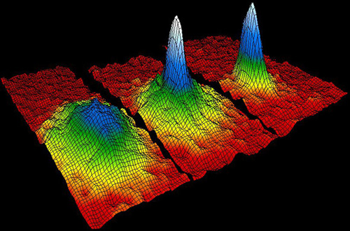
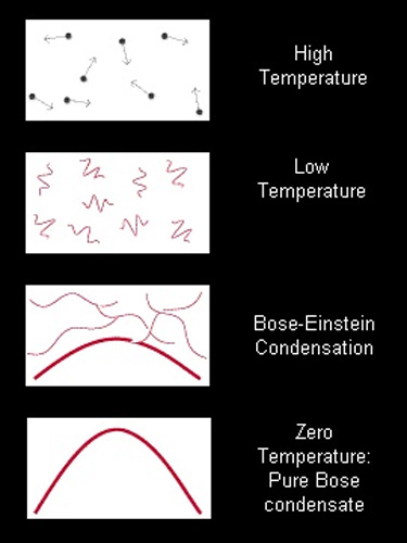
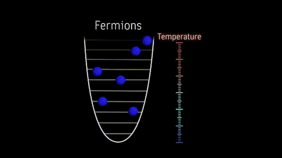
Figure 1: Some of the first experimental evidence for a gaseous macroscopic quantum state.
Source: © Mike Matthews, JILA.
Atomic physics experiments routinely trap clouds of atoms, as described in Unit 5, but the atoms in these gas clouds are all distinct entities with separate quantum mechanical wavefunctions. This unit will describe how it is possible for the wavefunctions of all the atoms to merge into a single, macroscopic quantum state. This occurs when the interactions between the atoms are exactly the right strength and the atoms are very cold. The figure above shows three false color images of trapped atoms. The fastest atoms are colored red, and as they slow down their colors change to yellow, green, blue, and finally white. Moving from left to right, the three images show successive stages of cooling leading to the majority of atoms being in a single macroscopic quantum state in the trap at a temperature of ~10-8 K. The 2001 Nobel Prize in physics was awarded to Carl Wieman, Eric Cornell, and Wolfgang Ketterle for first creating these special quantum gases in their laboratories. (Unit: 6)

We typically view quantum mechanics as applying only to the fundamental particles or fields of Units 1 and 2, and not to the objects we find in a grocery store or in our homes. If large objects like baseballs and our dining tables don’t behave like waves, why do we bother about their possible quantum nature? More practically, we can ask: If we are supposed to believe that ordinary objects consist of wave-like quantum particles, how does that quantum nature disappear as larger objects are assembled from smaller ones? Or, more interestingly: Are there macroscopic objects large enough to be visible to the naked eye that still retain their quantum wave natures? To answer these questions, we need the rules for building larger objects out of smaller ones, and the means of applying them. The rules are of a highly quantum nature; that is, they have no counterpart at all in classical physics, nor are they suggested by the behavior of the ordinary material objects around us. But in surprising ways, they lead to macroscopic quantum behavior, as well as the classical world familiar to all of us.

To interpret these rules, we need to understand two critical factors. First, particles of all types, including subatomic particles, atoms, molecules, and light quanta, fall into one of two categories: fermions and bosons. As we shall see, the two play by very different rules. Equally important, we will introduce the concept of pairing. Invoked more than a century ago to explain the creation of molecules from atoms, this idea plays a key role in converting fermions to bosons, the process that enables macroscopic quantum behavior. This unit will explore all these themes and Unit 8 will expand upon them.

Building up atoms and molecules

We start with the empirically determined rules for building atoms out of electrons, protons, and neutrons, and then move on to the build-up of atoms into molecules. The quantum concept of the Pauli exclusion principleplays a key role in this build-up (or, in the original German, aufbau). This principle prevents more than one fermion of the same fundamental type from occupying the same quantum state, whether that particle be in a nucleus, an atom, a molecule, or even one of the atom traps discussed in Unit 5. But the exclusion principle applies only to identical fermions. Electrons, neutrons, and protons are all fermions; but, although all electrons are identical, and thus obey an exclusion principle, they certainly differ from neutrons or protons, and these non-identical fermions are not at all restricted by the presence of one another. Chemists and physicists understood the exclusion principle’s empirical role in constructing the periodic table well before the discovery of the quantum theory of Unit 5; but they did not understand its mathematical formulation or its theoretical meaning.

Particles of light, or photons, are of a different type altogether: They are bosons, and do not obey the exclusion principle. Thus, identical photons can all join one another in precisely the same quantum state; once started, in fact, they are actually attracted to do so. This is the antithesis of the exclusion principle. Large numbers of such photons in the same quantum state bouncing back and forth between two mirrors several inches or even many meters apart create an essential part of a laser that, in a sense, is a macroscopic quantum system with very special properties.

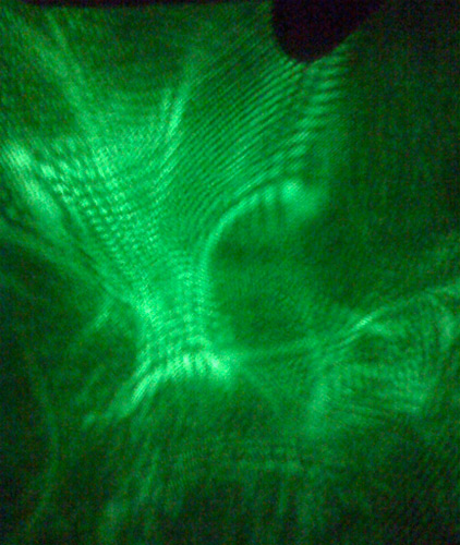
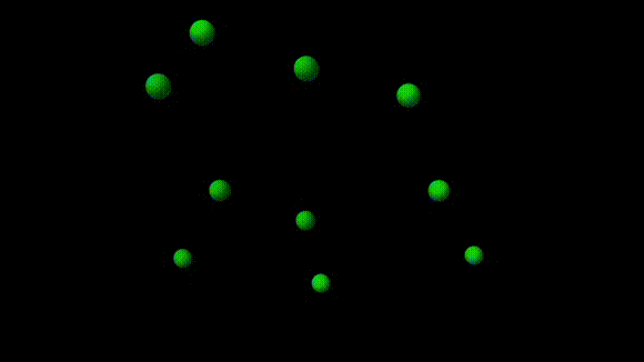
Figure 2: Diffraction of green laser light passing through a random medium.
Source: © William P. Reinhardt.
Photons in a laser are all in the same quantum state. The waves that correspond to individual photons are all in phase and, as we learned in Unit 5, will interfere when diffracted, for example, through a slit. The complicated interference pattern shown here is the result of shining a green laser into a randomly ordered transparent material. Photons interfere constructively and destructively after scattering within the material, resulting in a chaotic-looking pattern of bright and dark spots and lines. (Unit: 6)

Lasers are everywhere in our technology, from laser pointers to surgical devices and surveying equipment, to the inner workings of CD and DVD players. Laser light sent from telescopes and reflected from mirrors on the Moon allows measurement of the distance between the Earth and Moon to better than one millimeter, allowing tests of gravitational theory, measurement of the slowly increasing radius of the moon’s orbit around the Earth, and even allows geophysicists to observe the day-to-day motion of the continents (actually the relative motion of plate tectonics) with respect to one another: A bright light indeed. In addition to being bright and intense, laser light is coherent. Not only do all the particulate photons wave with the same wavelength (or color), but they are also shoulder-to-shoulder in phase with one another. This phase coherence of very large numbers of photons is a quantum property that follows from their bosonic nature. Yet, it persists up into the macroscopic world.

Superfluids and superconductors

Are there other macroscopic quantum systems in which actual particles (with mass) cooperate in the same coherent manner as the photons in a laser? We might use the molecules we will build up to make a dining room table, which has no evident quantum wave properties; so perhaps quantum effects involving very large numbers of atoms simply don’t persist at the macroscopic level or at room temperature. After all, light is quite special, as particles of light have no mass or weight. Of course, we fully expect light to act like a wave, it’s the particulate nature of light that is the quantum surprise. Can the wave properties of massive particles appear on a macroscopic scale?

The surprising answer is yes; there are macroscopic quantum systems consisting of electrons, atoms, and even molecules. These are the superfluids and superconductors of condensed matter physics and more recently the Bose condensates of atomic and molecular physics. Their characteristics typically appear at low (about 1–20 K), or ultra-low (about 10^-8 K and even lower) temperatures. But in some superconductors undamped currents persist at rather higher temperatures (about 80 K). These are discussed in Unit 8.

Superfluids are liquids or gases of uncharged particles that flow without friction; once started, their fluid motion will continue forever—not a familiar occurrence for anything at room temperature. Even super-balls eventually stop bouncing as their elasticity is not perfect; at each bounce, some of their energy is converted to heat, and eventually they lie still on the floor.

Figure 3: Superconducting magnets enable MRI machines to produce dramatic images.
Source: © Left: Wikimedia Commons, Creative Commons Attribution 3.0 Unported License. Author: Jan Ainali, 12 February 2008. Right: NIH.
On the left is a magnetic resonance imaging (MRI) apparatus in a hospital setting. Superconducting current flows produce the very high, sustained magnetic fields required to use the spins of protons in human tissue to create images like the brain scan on the right. Magnetic fields are easily generated from an electric current, but the current required for efficient MRI scanning generates a tremendous amount of heat. The solution is to use superconducting magnets, in which electric current can flow without resistance. The electrons in a superconductor are in a macroscopic quantum state that we will learn about in this unit and in Unit 8. As we delve further into the unit, the concept of spin, electrons, protons, and neutrons will come to play a crucial role in our understanding of the possibility of creating macroscopic quantum states, as well as for their dramatic use as a medical diagnostic tool. (Unit: 6)

Superconductors have this same property of flowing forever once started, except that they are streams of charged particles and therefore form electric currents that flow without resistance. As a flowing current generates a magnetic field, a superconducting flow around a circle or a current loop generates a possibly very high magnetic field. This field never dies, as the super-currents never slow down. Hospitals everywhere possess such superconducting magnets. They create the high magnetic fields that allow the diagnostic procedure called MRI (Magnetic Resonance Imaging) to produce images of the brain or other soft tissues. This same type of powerful superconducting magnetic field is akin to those that might levitate trains moving along magnetic tracks without any friction apart from air resistance. And as we saw in Unit 1, physicists at CERN’s Large Hadron Collider use superconducting magnets to guide beams of protons traveling at almost the speed of light.

Thus, there are large-scale systems with quantum behavior, and they have appropriately special uses in technology, engineering, biology and medicine, chemistry, and even in furthering basic physics itself. How does this come about? It arises when electrons, protons, and neutrons, all of which are fermions, manage to arrange themselves in such a way as to behave as bosons, and these composite bosons are then sucked into a single quantum state, like the photons in a laser.

Pairing and exclusion

What is required to create one of these composite quantum states, and what difference does it make whether the particles making up the state are fermions or bosons? Historically, the realization that particles of light behaved as bosons marked the empirical beginning of quantum mechanics, with the work of Planck, Einstein, and, of course, Bose, for whom the boson is named. In Unit 5, we encountered Planck’s original (completely empirical) hypothesis that the energy at frequency in an equilibrium cavity filled with electromagnetic radiation at temperature T should be n, where h is Planck’s constant, is the photon frequency, and n is a mathematical integer, say 0, 1, 2, 3…. Nowadays, we can restate the hypothesis by saying that n photons of energy hv are all in the same quantum mode, which is the special property of bosons. This could not happen if photons were fermions.

Another, at first equally empirical, set of models building up larger pieces of matter from smaller came from Dmitri Mendeleev’s construction and understanding of the periodic table of the chemical elements. American chemist G. N. Lewis pioneered the subsequent building up of molecules from atoms of the elements. His concept that pairs of electrons form chemical bonds and pairs and octets of electrons make especially stable chemical elements played a key role in his approach. This same concept of pairing arises in converting fermions into the bosons needed to become superconductors and superfluids, which will be our macroscopic quantum systems.

Figure 4: Early periodic table.
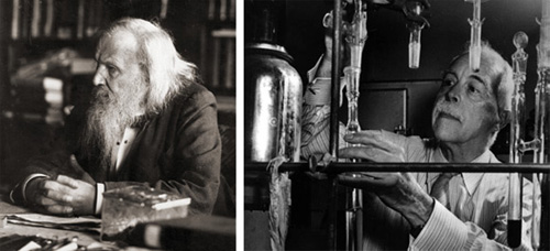
In the period around 1870, Dmitri Mendeleev, following and greatly extending the work of earlier chemists, arranged the chemical elements, whose composition was entirely unknown at the time, essentially in order of their increasing atomic mass. He noted that certain periodic properties occurred, which suggested that the elements not only should be listed, but also arranged in rows with elements having similar chemical and physical properties above or below one another. In doing so, he found gaps and misalignment, which suggested missing elements. Mendeleev famously predicted not only the existence of the elements which we now call “gallium,” “germanium,” and “technetium,” but quite accurately predicted many of their chemical and physical properties. (Unit: 6)

Austrian theorist Wolfgang Pauli took the next step. The theoretical development of modern quantum mechanics by Heisenberg and Schrödinger allowed him to make a clear statement of the exclusion principle needed to build up the periodic table of elements. That principle also made clear the distinction between fermions and bosons as will be discussed in Section 4. But first, we will address how models of atomic structure were built, based on the discovery of the electron and the atomic nucleus. Then we will follow the quantum modeling of the atom, explaining these same empirical ideas once the quantum theory of Unit 5 is combined with Pauli’s exclusion principle.

The foundation for all that follows is the periodic table that Russian chemist Dmitri Mendeleev formulated by arranging the chemical elements in order of their known atomic weights. The table not only revealed the semi-periodic pattern of elements with similar properties, but also contained specific holes (missing elements, see Figure 4) that allowed Mendeleev to actually predict the existence and properties of new chemical elements yet to be discovered. The American chemist G. N. Lewis then created an electron shell model giving the first physical underpinning of both Mendeleev’s table and of the patterns of chemical bonding. This is very much in the current spirit of particle physics and the Standard Model: symmetries, “magic numbers,” and patterns of properties of existing particles that strongly suggest the existence of particles, such as the Higgs boson, yet to be discovered.

Figure 5: The father and son of chemical periodicity: Mendeleev and Lewis.
Source: © Left: Wikimedia Commons, Public Domain. Right: Lawrence Berkeley National Laboratory.
in the period around 1870, Dmitri Mendeleev (left) created the first periodic table by arranging the chemical elements in a manner not only useful for understanding the relationships between the elements, but also for predicting the existence of as yet undiscovered elements. Gilbert Newton Lewis (right) developed an empirical shell model in the period from 1902 to 1916. Using data based on the periodic table and the observed bonding properties of the atomic elements to form molecules, Lewis proposed that it was the electrons in atoms that gave rise to their physical and chemical properties. In doing so, he developed the idea of filled shells (or kernels, as he called them) of two, and then eight, electrons as leading to special stability, and also the idea of the shared pair covalent bond, which are discussed later in this unit. (Unit: 6)

When Mendeleev assembled his periodic table in 1869, he was the giant standing on the shoulders of those who, in the 6 decades before, had finally determined the relative masses of the chemical elements, and the formulae of those simple combinations of atoms that we call “molecules.” In this arduous task, early 19th century chemists were greatly aided by using techniques developed over several millennia by the alchemists, in their attempts to, say, turn lead into gold. This latter idea, which nowadays seems either antiquated or just silly, did not seem so to the alchemists. Their view is reinforced by the realization that even as Mendeleev produced his table: No one had any idea what the chemical elements, or atoms as we now call them, were made of. Mendeleev’s brilliant work was empiricism of the highest order. John Dalton, following Democrates, had believed that they weren’t made of anything: Atoms were the fundamental building blocks of nature, and that was all there was to it.

Figure 6: Plum pudding (or raisin scone) model of the atom.
Source: © William P. Reinhardt, 2010.

This all began to change with J. J. Thomson’s discovery of the electron in 1897, and his proposed atomic model. Thomson found that atoms contained electrons, each with a single unit of negative charge. To his great surprise he also found that electrons were very light in comparison to the mass of the atoms from which they came. As atoms were known to be electrically neutral, the rest of the atom then had to be positively charged and contain most of the mass of the atom. Thomson thus proposed his plum pudding model of the atom.

Rutherford and Lewis

Thomson’s model was completely overthrown, less than 15 years later, by Ernest Rutherford’s discovery that the positive charge in an atom was concentrated in a very small volume which we now call the “atomic nucleus,” rather than being spread out and determining the size of the atom, as suggested by Thomson’s model. This momentous and unexpected discovery completely reversed Thomson’s idea: Somehow, the negatively charged electrons were on the outside of the atom, and determined its volume, just the opposite of the picture in Figure 6. How can that be?

The fact that electrons determine the physical size of an atom suggested that they also determine the nature of atomic interactions, and thus the periodic nature of chemical and physical interactions as summarized in Mendeleev’s Table, a fact already intuited by Lewis, based on chemical evidence. At ordinary energies, and at room temperature and lower, nuclei never come into contact. But, then one had to ask: How do those very light electrons manage to fill up almost all of the volume of an atom, and how do they determine the atom’s chemical and physical properties?

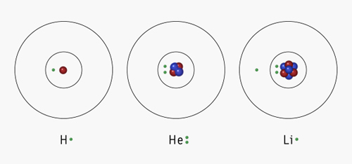
Figure 7: The Lewis shell model for the first three atoms in the modern periodic table.

A start had already been made. In 1902, when Rutherford’s atomic nucleus was still almost a decade in the future, American chemist G. N. Lewis, had already proposed an empirically-developed shell model to explain how electrons could run the show, even if he was lacking in supplying a detailed model of how they actually did so.

He suggested that the first atomic shell (or kernel as he originally called it) held two electrons at maximum, the second and third shells a maximum of eight, and the fourth up to 18 additional electrons. Thus, for neutral atoms and their ion, the “magic numbers” 2, 8, 8, and 18 are associated with special chemical stability. Electrons in atoms or ions outside of these special closed shells are referred to as valence electrons, and determine much of the physical and chemical behavior of an atom. For example, in Unit 8, we will learn that atoms in metallic solids lose their valence electrons, and the remaining ionic cores form a metallic crystal, with the former valence electrons moving freely like water in a jar of beads, and not belonging to any specific ion. In doing so, they may freely conduct electrical currents (and heat), or under special circumstances may also become superconductors, allowing these free electrons to flow without resistance or energy dissipation.

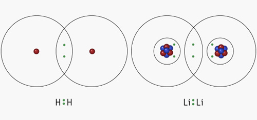
Lewis also assumed that chemical bonding took place in such a way that stable molecules had fully filled shells, and that they formed these full shells by sharing electrons in pairs. The simplest example is the formation of the hydrogen molecule. He denoted a hydrogen atom by H•, where the • is the unpaired electron in the atom’s half-filled first shell. Why two atoms in a hydrogen molecule? The answer is easy in Lewis’s picture: H:H. This pair of dots denotes that two shared electrons form the bond that holds the H₂ molecule together, where the subscript means that the molecule consists of two hydrogen atoms. As there are now no longer any unpaired electrons, we don’t expect to form H₃ or H₄. Similarly, helium, which already has the filled shell structure He:, has no unpaired electrons to share, so does not bond to itself or to other atoms.

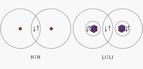
Figure 8: Molecules in the Lewis shell picture: the pair bond for H2 and Li2.
The diagrams above illustrate the Lewis picture of chemical covalent bonds as shared pairs of electrons. On the left, we have a hydrogen molecule, in which two hydrogen atoms share the single electron in their first shell, thus attaining the magic number two for a stable, filled first shell. On the right, lithium atoms, each with a single electron outside an inner already filled shell, can also form a single pair bond. As in the shell diagrams for single atoms, these molecular diagrams are useful for illustrating how certain molecules form. However, they are not, by any means, schematic diagrams of what molecules actually look like. (Unit: 6)

Next, Lewis introduced his famous counting rule (still used in models of bonding in much of organic chemistry and biochemistry): As the electrons are shared in overlapping shells, we count them twice in the dot picture for H₂, one pair for each H atom. Thus, in the Lewis manner of counting, each H atom in H₂ has a filled shell with two electrons just like Helium: He:. Here, we have the beginning of the concept of pairs or pairing, albeit in the form of a very simple empirical model. Such pairings will soon dominate all of our discussion.

How can those tiny electrons determine the size of an atom?

Lewis’s model implies certain rules that allow us to understand how to build up an atom from its parts, and for building up molecules from atoms, at least for the electrons that determine the structure of the periodic table and chemical bonding. Another set of such rules tells us how to form the nucleus of an atom from its constituent neutrons and protons. The formation of nuclei is beyond the scope of this unit, but we should note that even these rules involve pairing.

We can take such a blithe view of the structure of the nucleus because this first discussion of atoms, molecules, solids, and macroscopic quantum systems involves energies far too low to cause us to worry about nuclear structure in any detail. It is the arrangement of and behavior of the electrons with respect to a given nucleus, or set of nuclei, that determines many of the properties of the systems of interest to us. However, we should not forget about the nucleus altogether. Once we have the basic ideas involving the structure of atoms and molecules at hand, we will ask whether these composite particles rather than their constituent parts are bosons or fermions. When we do this, we will suddenly become very interested in certain aspects of the nucleus of a given atom. But, the first critical point about the nucleus in our initial discussion involves its size in comparison with that of the atom of which it is, somehow, the smallest component.

Figure 9: Rutherford’s model of a hydrogen atom.
Source: © Wikimedia Commons, Public Domain. Author: Bensaccount, 10 July 2006.
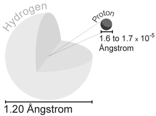
In the Rutherford model of the atom, the positive charge and most of the mass of an ordinary hydrogen atom, consisting of one electron and one proton, is that of the proton, which has a linear diameter about 10-5 smaller than the size of the atom itself. Thus, the volume of the nucleus is 1015 times smaller than the volume of the entire atom. As an electron by itself has essentially no intrinsic volume, it is common to say that an atom is mostly empty space. What, then, creates and determines the actual size of the atom? We will see that the answer is quantum mechanics, which, as it turns out fortuitously, also lays out the entire structure of the periodic table. (Unit: 6)

Although it contains almost all of the atom’s mass and its entire positive electrical charge, the nucleus is concentrated in a volume of 1 part in 10¹⁵ (that’s one thousand trillion) of the physical volume of the atom. The size of the atom is determined by the electrons, which, in turn, determine the size of almost everything, be it solid or liquid, made of matter that we experience in daily life. For example, the volume of water in a glass of water is essentially the volume of the atoms comprising the water molecules that fill the glass. However, if the water evaporates or becomes steam when heated, its volume is determined by the size of the container holding the gaseous water. That also applies to the gaseous ultra-cold trapped atoms that we first met in Unit 5 and will encounter again later in this unit as Bose-Einstein condensates (BECs). They expand to fill the traps that confine them. How is it that these negatively charged and, in comparison to nuclei, relatively massless electrons manage to take up all that space?

Atoms and their nuclei

The atomic nucleus consists of neutrons and protons. The number of protons in a nucleus is called the atomic number, and is denoted by Z. The sum of the number of protons and neutrons is called the mass number, and is denoted by A. The relation between these two numbers Z and A will be crucial in determining whether the composite neutral atom is a boson or fermion. The volume of a nucleus is approximately the sum of the volumes of its constituent neutrons and protons, and the nuclear mass is approximately the sum of the masses of its constituent neutrons and protons. The rest of the atom consists of electrons, which have a mass of about 1/2,000 of that of a neutron or proton, and a negative charge of exactly the same magnitude as the positive charge of the proton. As suggested by its name, the neutron is electrically neutral. The apparently exact equality of the magnitudes of the electron and proton charges is a symmetry of the type we encountered in Units 1 and 2.

Do electrons have internal structure?

Now back to our earlier question: How can an atom be so big compared to its nucleus? One possibility is that electrons resemble big cotton balls of negative charge, each quite large although not very massive, as shown in Figure 10 below. As they pack around the nucleus, they take up lots of space, leading to the very much larger volume of the atom when compared to the volume of the nucleus.

Figure 10: A cotton ball model of an atom.
Source: © William P. Reinhardt
A conceptual model of the atom suggests that electrons are like fluffy balls of cotton, each repelled by the Coulomb repulsion of other electrons, but held together by the large positive charge on the small but massive nucleus at the center of the atom. This figure brings a three-dimensional reality to the flat-looking Lewis dot diagrams of earlier representations, and it is not necessarily at odds with the quantum models of the atom we will soon be discussing. The difference will be in the interpretation of the cotton balls. (Unit: 6)

However, there is a rather big problem with the simple cotton ball idea. When particle physicists try to measure the radius or volume of an individual electron, the best answer they get is zero. Said another way, no measurement yet made has a spatial resolution small enough to measure the size of an individual electron thought of as a particle. We know that electrons are definitely particles. With modern technology we can count them, even one at a time. We also know that each electron has a definite amount of mass, charge, and—last, but not at all least, as we will soon see—an additional quantity called spin. In spite of all this, physicists still have yet to observe any internal structure that accounts for these properties.

It is the province of string theory, or some yet-to-be created theory with the same goals, to attempt to account for these properties at length scales far too small for any current experiments to probe. Experimentalists could seek evidence that the electron has some internal structure by trying to determine whether it has an electric dipole moment. Proof of such a moment would mean that the electron’s single unit of fundamental negative charge is not uniformly distributed within the electron itself. Since the Standard Model introduced in Unit 1 predicts that the electron doesn’t have a dipole moment, the discovery of such an internal structure would greatly compromise the model.

For now, though, we can think of an electron as a mathematical point. So how do the electrons take up all the space in an atom? They certainly are not the large cotton balls we considered above; that would make everything too simple, and we wouldn’t need quantum mechanics. In fact we do need quantum mechanics in many ways. Ironically, the picture that quantum mechanics gives, with its probability interpretation of an atomic wavefunction, will bring us right back to cotton balls, although not quite those of Figure 10.

Figure 11: A simple classical model fails to explain the stability of the helium atom.
Source: © William P. Reinhardt, 2010.
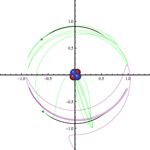
Bohr’s classical orbits astonishingly allowed him to predict the actual energy levels, and spectra, of the electron in the one-electron hydrogen atom, but what happens when there are two electrons? In 1921, Irving Langmuir found periodic orbits of two electrons moving with respect to a fixed nucleus (which is not drawn to scale here). In these periodic orbits, the repelling electrons bounce back and forth along the black paths shown above. However, this orbit is completely unstable. If one of the electrons is slightly disturbed, the electrons immediately follow chaotic trajectories such as the ones shown by the green and purple lines. One electron is ejected from the atom, and the other remains in a stable orbit around the nucleus. As helium atoms are the most stable atoms known, and by no means self-ionize, this indicates that classical motion of the electrons is only a good starting point for understanding the nature of atomic structure and spectra for one-electron atoms and ions. In fact, we actually need quantum mechanics to fully understand the hydrogen atom, and most definitely to understand even the most basic properties of the helium atom. (Unit: 6)

As we learned in Unit 5, quantum theory replaces Bohr’s orbits with standing, or stationary state, wavefunctions. Just as in the Bohr picture, each wavefunction corresponds to the possibility of having the system, such as an electron in an atom, in a specific and definite energy level. As to what would happen when an atom contained more than one electron, Bohr was mute. Astronomers do not need to consider the interactions between the different planets in their orbits around the Sun in setting up a first approximation to the dynamics of the solar system, as their gravitational interactions with each other are far weaker than with the Sun itself.

The Sun is simply so massive that to a good first approximation it controls the motions of all the planets. Bohr recognized that the same does not apply to the classical motion of electrons in the next most complex atom: Helium, with a charge of +2 on its nucleus and two moving electrons. The electrons interact almost as strongly with each other as with the nucleus that holds the whole system together. In fact, most two-electron classical orbits are chaotically unstable, causing theoretical difficulties in reconciling the classical and quantum dynamics of helium that physicists have overcome only recently and with great cleverness.

Perhaps surprisingly, the energy levels described by Schrödinger’s standing wave picture very quickly allowed the development of an approximate and qualitative understanding of not only helium, but most of the periodic table of chemical elements.

Energy levels for electrons in atoms

What is the origin of the Lewis filled shell and electron pair bonding pictures? It took the full quantum revolution described in Unit 5 to find the explanation—an explanation that not only qualitatively explains the periodic table and the pair bond, but also gives an actual theory that allows us to make quantitative computations and predictions.

When an atom contains more than one electron, it has different energies than the simple hydrogen atom; we must take both the quantum numbers n (from Unit 5) and l (which describes a particle’s quantized angular momentum), into account. This is because the electrons do not move independently in a many-electron atom: They notice the presence of one another. They not only affect each other through their electrical repulsion, but also via a surprising and novel property of the electron, its spin, which appeared in Unit 5 as a quantum number with the values ±1/2, and which controls the hyperfine energies used in the construction of phenomenally accurate and precise atomic clocks.

The effect of electron spin on the hyperfine energy is tiny, as the magnetic moment of the electron is small. On the other hand, when two spin-1/2 electrons interact, something truly incredible happens if the two electrons try to occupy the same quantum state: In that case, one might say that their interaction becomes infinitely strong, as they simply cannot do it. So, if we like, we can think of the exclusion principle mentioned in the introduction to this unit as an extremely strong interaction between identical fermions.

Figure 12: The ground state of helium: energy levels and electron probability distribution.
The diagram on the left shows the energy levels that electrons in helium are allowed to occupy as horizontal lines. Energy levels with the quantum number l = 0, shown in black, can contain two electrons. Energy levels with l = 1, shown in blue, can contain six electrons. To get the ground state of the helium atom, we put one spin-up and one spin-down electron into the lowest available energy level. The image on the right is the electron probability density in a helium atom in its ground state. In the quantum mechanical atom, we cannot know what the two electrons are doing at any instant in time. We only know the probability of finding one of them at a given point in space. The probability density cloud is centered on the nucleus, and the darker shade of blue indicates regions of higher probability. The presence of the two electrons will cause the charge probability density cloud shown in the right half of the figure to expand; but this is then offset by the fact that the nucleus now contains two, rather than one, positively charged protons. This larger nuclear charge ends up causing the size of helium to actually be smaller than that of the hydrogen atom. (Unit: 6)

We are now ready to try building the periodic table using a simple recipe: To get the lowest energy, or ground state of an atom, place the electrons needed to make the appropriate atomic or ionic system in their lowest possible energy levels, noting that two parallel spins can never occupy the same quantum state. This is called the Pauli exclusion principle. Tradition has us write spin +1/2 as ↑ and spin -1/2 as ↓, and these are pronounced “spin up” and “spin down.” In this notation, the ground state of the He atom would be represented as n = 1 and ↑↓, meaning that both electrons have the lowest energy principal quantum number n = 1, as in Unit 5, and must be put into that quantum state with opposite spin projections.

Quantum mechanics also allows us to understand the size of atoms, and how seemingly tiny electrons take up so much space. The probability density of an electron in a helium atom is a balance of three things: its electrical attraction to the nucleus, its electrical repulsion from the other electron, and the fact that the kinetic energy of an electron gets too large if its wavelength gets too small, as we learned in Unit 5. This is actually the same balance between confinement and kinetic energy that allowed Bohr, with his first circular orbit, to also correctly estimate the size of the hydrogen atom as being 10⁵ times larger than the nucleus which confines it.

Assigning electrons to energy levels past H and He

Now, what happens if we have three electrons, as in the lithium (Li) atom? Lewis would write Li•, simply not showing the inert inner shell electrons. Where does this come from in the quantum mechanics of the aufbau? Examining the energy levels occupied by the two electrons in the He atom shown in Figure 12 and thinking about the Pauli principle make it clear that we cannot simply put the third electron in the n = 1 state. If we did, its spin would be parallel to the spin of one of the other two electrons, which is not allowed by the exclusion principle. Thus the ground state for the third electron must go into the next lowest unoccupied energy level, in this case n = 2, l = 0.

Figure 13: Electrons in atomic energy levels for Li, Na, and K
This aufbau for the first three rows of the periodic table follows the Pauli exclusion principle, in that the lowest energy levels are each occupied by two electrons of opposite spin before higher lying levels fill in. The diagrams above show the allowed electron energies as horizontal lines, and represent electrons as arrows that indicate whether the electron is spin-up or spin-down. We see that the Li atom (left) has an unpaired outermost electron in the n = 2, l = 0 state; for Na (center) and K (right), this is replaced by the outer electron being in the n = 3, l = 0 and n = 4, l = 0 states, respectively. These single unpaired electrons outside an inert filled shell impart similar physical and chemical properties to these three elements, which are all in the first column of the periodic table. (Unit: 6)

Using the exclusion principle to determine electron occupancy of energy levels up through the lithium (Li), sodium (Na), and potassium (K) atoms, vindicates the empirical shell structures implicit in the Mendeleev table and explicit in Lewis’s dot diagrams. Namely Li, Na, and K all have a single unpaired electron outside of a filled (and thus inert and non-magnetic) shell. It is these single unpaired electrons that allow these alkali atoms to be great candidates for making atomic clocks, and for trapping and making ultra-cold gases, as the magnetic traps grab that magnetic moment of that unpaired electron.

Where did this magical Pauli exclusion principle come from? Here, as it turns out, we need an entirely new, unexpected, and not at all intuitive fundamental principle. With it, we will have our first go-around at distinguishing between fermions and bosons.

In spite of having no experimentally resolvable size, a single electron has an essential property in addition to its fixed charge and mass: a magnetic moment. It may line up, just like a dime store magnet, north-south or south-north in relation to a magnetic field in which it finds itself. These two possible orientations correspond to energy levels in a magnetic field determined by the magnet’s orientation. This orientation is quantized in the magnetic field. It turns out, experimentally, that the electron has only these two possible orientations and energy levels in a magnetic field. The electron’s magnetic moment is an internal and intrinsic property. For historical reasons physicists called it spin, in what turned out to be a bad analogy to the fact that in classical physics a rotating spherical charge distribution, or a current loop as in a superconducting magnet, gives rise to a magnetic moment. The fact that only two orientations of such a spin exist in a magnetic field implies that the quantum numbers that designate spin are not integers like the quantum numbers we are used to, but come in half-integral amounts, which in this case are 1/2. This was a huge surprise when it was first discovered.

Figure 14: The Stern-Gerlach experiment demonstrated that spin orientation is quantized, and that “up” and “down” are the only possibilities.
Source: © Wikimedia Commons, GNU Free Documentation License, Version 1.2. Author: Peng, 1 July 2005

What does this mean? A value of 1/2 for the spin of the electron pops out of British physicist Paul Dirac’s relativistic theory of the electron; but even then, there is no simple physical picture of what the spin corresponds to. Ask a physicist what “space” spin lives in, and the answer will be simple: Spins are mathematical objects in “spin space.” These spins, if unpaired, form little magnets that can be used to trap and manipulate the atoms, as we have seen in Unit 5, and will see again below. But spin itself has much far-reaching implications. The idea of “spin space” extends itself into “color space,” “flavor space,” “strangeness space,” and other abstract (but physical, in the sense that they are absolutely necessary to describe what is observed as we probe more and more deeply into the nature of matter) dimensions needed to describe the nature of fundamental particles that we encountered in Units 1 and 2.

Spin probes of unusual environments

Is spin really important? Or might we just ignore it, as the magnetic moments of the proton and electron are small and greatly overwhelmed by their purely electrical interactions? In fact, spin has both straightforward implications and more subtle ones that give rise to the exclusion principle and determine whether composite particles are bosons or fermions.

The more direct implications of the magnetic moments associated with spin include two examples in which we can use spins to probe otherwise hard-to-reach places: inside our bodies and outer space. It turns out that the neutron and proton also have spin-1/2 and associated magnetic moments. As these magnetic moments may be oriented in only two ways in a magnetic field, they are usually denoted by the ideograms ↑ and ↓ for the spin projections +1/2 (spin up) and -1/2 (spin down). In a magnetic field, the protons in states ↑ and ↓ have different energies. In a strong external magnetic field, the spectroscopy of the transitions between these two levels gives rise to Nuclear Magnetic Resonance (NMR), a.k.a. MRI in medical practice (see Figure 3). Living matter contains lots of molecules with hydrogen atoms, whose nuclei can be flipped from spin up to spin down and vice versa via interaction with very low energy electromagnetic radiation, usually in the radiowave regime. The images of these atoms and their interactions with nearby hydrogen atom nuclei provide crucial probes for medical diagnosis. They also support fundamental studies of chemical and biochemical structures and dynamics, in studies of the folding and unfolding of proteins, for example.

Another example of the direct role of the spins of the proton and electron arises in astrophysics. In a hydrogen atom, the spin of the proton and electron can be parallel or anti-parallel. And just as with real magnets, the configuration(p(↑)(↓) has lower energy than p(↑)e(↓). This small energy difference is due to the hyperfine structure of the spectrum of the hydrogen atom reviewed in Unit 5. The photon absorbed in the transition p(↑)e(↓)→p(↑)e(↑) or emitted in the transition p(↑)e(↑)→p(↑)e(↓) has a wavelength of 21 centimeters, in the microwave region of the electromagnetic spectrum. Astronomers have used this 21 centimeter radiation to map the density of hydrogen atoms in our home galaxy, the Milky Way, and many other galaxies.

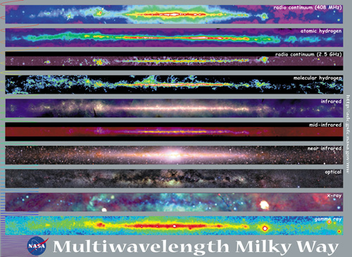
Figure 15: Our galaxy, imaged at many different wavelengths.
Source: © NASA.
Astronomers and astrophysicists use many tools to gain information about the structure and properties of our own galaxy, the Milky Way. This diagram shows radiation emitted by objects in the Milky Way from very long wavelength, low-energy radiation (top) to very short wavelength, high-energy radiation (bottom). Atomic hydrogen is observed using the spin-flip 21 cm radiation discussed in the text, giving the map of hydrogen in the galaxy that appears second from the top. All of the images show our galaxy “edge on” as we are within the galaxy itself, and have, as yet, no way to collect data giving other perspectives or viewpoints. These are easily obtained for faraway galaxies, as many of these are similar to our own, and are observed in random orientations with respect to ours. (Unit: 6)

Electrons are fermions

However, there is more: That a particle has spin 1/2 means more than that it has only two possible orientations in a magnetic field. Fundamental particles with intrinsic spin of 1/2 (or any other half-integer spin, such as 3/2 or 5/2 or more whose numerators are odd numbers) share a specific characteristic: They are all fermions; thus electrons are fermions. In contrast, fundamental particles with intrinsic spin of 0, 1, 2, or any integral number are bosons; so far, the only boson we have met in this unit is the photon.

Is this a big deal? Yes, it is. Applying a combination of relativity and quantum theory, Wolfgang Pauli showed that identical fermions or bosons in groups have very different symmetry properties. No two identical fermions can be in the same quantum state in the same physical system, while as many identical bosons as one could wish can all be in exactly the same quantum state in a single quantum system. Because electrons are fermions, we now know the correct arrangement of electrons in the ground state of lithium. As electrons have only two spin orientations, ↑ or ↓, it is impossible to place all three electrons in the lowest quantum energy level; because at least two of the three electrons would have the same spin, the state is forbidden. Thus, the third electron in a lithium atom must occupy a higher energy level. In recognition of the importance of spin, the Lewis representation of the elements in the first column of the periodic table might well be H↑, Li↑, Na↑, K↑, and Rb↑, rather than his original H^•, Li^•, Na^•, K^•, and Rb^•. The Pauli symmetry, which leads to the exclusion principle, gives rise to the necessity of the periodic table’s shell structure. It is also responsible for the importance of Lewis’s two electron chemical pair bond, as illustrated in Figure 16.

Figure 16: Spin pairing in the molecules H₂ and Li₂.
The Pauli exclusion principle requires that two electrons in the same spatial standing wave quantum state have opposite spins. This is illustrated for the covalent pair bonding electrons in H2 and Li2, and also for the pairs of electrons in the inner helium-like shells of the Li atoms. Thus, the pairing of electrons of opposite spins allows formation of the strong bonds enabling atoms to join to form molecules, as well as determining the number of electrons contained in inner atomic shells. If the bonding electrons have parallel spins, the bonding will be far weaker, or not even take place. (Unit: 6)

The Pauli rules apply not only to electrons in atoms or molecules, but also to bosons and fermions in the magnetic traps of Unit 5. These may be fundamental or composite particles, and the traps may be macroscopic and created in the laboratory, rather than electrons attracted by atomic nuclei. The same rules apply.

Conversely, the fact that bosons such as photons have integral spins means that they can all occupy the same quantum state. That gives rise to the possibility of the laser, in which as many photons as we wish can bounce back and forth between two mirrors in precisely the same standing wave quantum state. We can think of this as a macroscopic quantum state. This is certainly another example of particles in an artificial trap created in the laboratory, and an example of a macroscopic quantum state. Lasers produce light with very special and unusual properties. Other bosons will, in fact, be responsible for all the known macroscopic quantum systems that are the real subject of this and several subsequent units.

Photons are bosons

When Max Planck introduced the new physical constant h that we now call blackbody">Planck’s constant[./tooltip], he used it as a proportionality constant to fit the data known about blackbody radiation, as we saw in Unit 5. It was Albert Einstein who noted that the counting number n that Planck used to derive his temperature dependent emission profiles was actually counting the number of light quanta, or photons, at frequency v, and thus that the energy of one quantum of light was hv. If one photon has energy hv, then n photons would have energy n. What Planck had unwittingly done was to quantize electromagnetic radiation into energy packets. Einstein and Planck both won Nobel prizes for this work on quantization of the radiation field.

What neither Planck nor Einstein realized at the time, but which started to become clear with the work of the Indian physicist Satyendra Bose in 1923, was that Planck and Einstein had discovered that photons were a type of particle we call “bosons,” named for Bose. That is, if we think of the frequency as describing a possible mode or quantum state of the Planck radiation, then what Planck’s n really stated was that any number, n = 0, 1, 2, 3…, of photons, each with its independent energy hv could occupy the same quantum state.

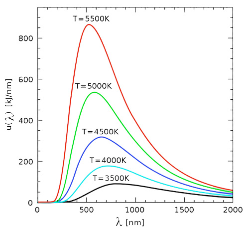
Figure 17: The spectrum of blackbody radiation at different temperatures.
Source: © Wikimedia Commons, GNU Free Documentation license, Version 1.2. Author: 4C, 04 August 2006
In Unit 5, we learned that a blackbody at a particular temperature emits radiation according to the Planck distribution. As shown here, black bodies at higher temperatures produce more of this radiant energy, and the peak of the spectrum is shifted to energies that correspond to shorter wavelengths. An essential part of the derivation of these results, which are in excellent agreement with the experiment, was Planck’s (implicit!) bosonic assumption that n quanta of light could occupy a mode at frequency, v. (Unit: 6)

In the following year, Einstein also suggested in a second paper following the work of Bose, that atoms or molecules might be able to behave in a similar manner: Under certain conditions, it might be possible to create a gas of particles all in the same quantum state. Such a quantum gas of massive particles came to be known as a Bose-Einstein condensate (BEC) well before the phenomenon was observed. Physicists observed the first gaseous BEC 70 years later, after decades of failed attempts. But, in 1924, even Einstein didn’t understand that this would not happen for just any atom, but only for those atoms that we now refer to as bosons. Fermionic atoms, on the other hand, would obey their own exclusion principle with respect to their occupation of the energy levels of motion in the trap itself.

Whether atoms and molecules can condense into the same quantum state, as Einstein predicted in 1924, depends on whether they are bosons or fermions. We therefore have to extend Pauli’s definition of bosons and fermions to composite particles before we can even talk about things as complex as atoms being either of these. As a start, let’s consider a composite object made from two spin-1/2 fundamental particles. The fundamental particles are, of course, fermions; but when we combine them, the total spin is either  1/2 + 1/2=1 or 1/2 – 1/2=0. This correctly suggests that two spin-1/2 fermions may well combine to form a total spin of 1 or 0. In either case, the integer spin implies that the composite object is a boson.

Why the caveat “may well”? As in many parts of physics, the answer to this question depends on what energies we are considering and what specific processes might occur. We can regard a star as a structureless point particle well described by its mass alone if we consider the collective rotation of billions of such point masses in a rotating galaxy. However, if two stars collide, we need to consider the details of the internal structure of both. In the laboratory, we can think of the proton (which is a composite spin-1/2 fermion) as a single, massive, but very small and inert particle with a positive unit charge, a fixed mass, and a spin of 1/2 at low energies. But the picture changes at the high energies created in the particle accelerators we first met in Unit 1. When protons moving in opposite directions at almost the speed of light collide, it is essential to consider their internal structures and the new particles that may be created by the conversion of enormous energies into mass. Similarly two electrons might act as a single boson if the relevant energies are low enough to allow them to do so, and if they additionally have some way to actually form that composite boson; this requires the presence of “other particles,” such as an atomic nucleus, to hold them together. This also usually implies low temperatures. We will discuss electrons paired together as bosons below and in Unit 8. A hydrogen atom, meanwhile, is a perfectly good boson so long as the energies are low compared to those needed to disassemble the atom. This also suggests low temperatures. But, in fact, Einstein’s conditions for Bose condensation require extraordinarily low temperatures.

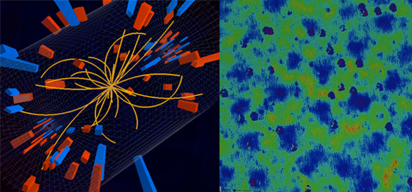
Figure 18: Protons in LHC collisions (left) and electrons in a superconductor (right) are examples of composite fermions and bosons.
The protons that came together in the LHC collision shown on the left are composite fermions made of three spin-1/2 quarks. Most protons we encounter in our daily lives behave as single composite fermions, no questions asked. However, collisions at the LHC and other particle accelerators are energetic enough that the proton’s internal structure cannot be ignored. At the opposite end of the energy scale are the electrons in superconductors, such as the one pictured on the right, which must be cooled well below room temperature. We normally think of electrons as individual spin-1/2 particles, but in a superconductor the electrons are paired up into bosons. It is these bosonic pairs that determine the electrical properties of the superconductor. (Unit: 6)

Helium as boson or fermion

When is helium a boson? This is a more complex issue, as the helium nucleus comes in two isotopes. Both have Z = 2, and thus two protons and two electrons. However, now we need to add the neutrons. The most abundant and stable form of helium has a nucleus with two protons and two neutrons. All four of these nucleons are spin-1/2 fermions, and the two protons pair up, as do the two neutrons. Thus, pairing is a key concept in the structure of atomic nuclei, as well as in the organization of electrons in the atom’s outer reaches. So, in helium with mass number A = 4, the net nuclear spin is 0. Thus, the ⁴He nucleus is a boson. Add the two paired electrons and the total atomic spin remains 0. So, both the nucleus and an atom of helium are bosons.

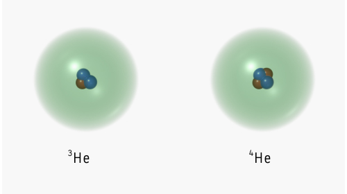
Figure 19: The two isotopes of helium: a fermion and a boson.
Helium has two stable, naturally occurring isotopes. The defining characteristic of helium is two protons in the nucleus, for an atomic number Z = 2. However, the helium nucleus can contain different numbers of neutrons. On the left we have 3He, with two protons, one neutron, and an atomic mass number A = 3. On the right we have 4He, with two protons, two neutrons, and A = 4. As both neutrons and protons are spin-1/2 fermions, the A = 3 nucleus is a fermion, and the A = 4 nucleus is a boson. In each case, the electron density cloud of a neutral helium atom contains a pair of spin-1/2 electrons. All possible arrangements of the two electrons in both isotopes result in a total electron spin of either 0 or 1, so the electrons form a bosonic pair in either case. Thus, when we add electronic and nuclear spins, we find that atomic 4He is a boson, and 3He, a fermion. (Unit: 6)

The chemical symbol He tells us that Z = 2. But we can add the additional information that A=4 by writing the symbol for bosonic helium as ⁴He, where the leading superscript 4 designates the atomic number. This extra notation is crucial, as helium has a second isotope. Because different isotopes of the same element differ only in the number of neutrons in the nucleus, they have different values of A. The second stable isotope of helium is ³He, with only one neutron. The isotope has two paired protons and two paired electrons but one necessarily unpaired neutron. ³He thus has spin-1/2 overall and is a composite fermion. Not surprisingly, ³He and ⁴He have very different properties at low temperatures, as we will discuss in the context of superfluids below.

Atomic bosons and fermions

More generally, as the number of spin-1/2 protons equals the number of spin-1/2 electrons in a neutral atom, any atom’s identity as a composite fermion or boson depends entirely on whether it has an odd or even number of neutrons, giving a Fermi atom and a Bose atom, respectively. We obtain that number by subtracting the atomic number, Z, from the mass number, A. Note that A is not entirely under our control. Experimentalists must work with the atomic isotopes that nature provides, or they must create novel ones, which are typically unstable; which isotopes these are depends on the rules for understanding the stability of nuclei. A difficult task as neutrons and protons interact in very complex ways, which befits their composite nature, and are not well represented by simple ideas like the electrical Coulomb’s Law attraction of an electron for a proton.

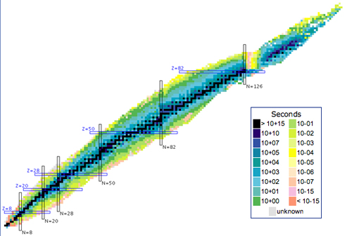
Figure 20: As this chart shows, not every imaginable nucleus is stable.
Source: © Courtesy of Brookhaven National Laboratory.

The mass number, A, of atoms is not entirely under our control, as this chart of nuclides shows. Each colored dot on the chart represents a nucleus either found in nature or created in the laboratory, with atomic number Z on the vertical axis, and mass number A (or N) on the horizontal axis. The color of the dot indicates the half-life of each nucleus: how long it lasts, on average, before decaying into another element. The darkest dots represent elements that we encounter in daily life, and the pink dots represent elements that last for less than 10-15 seconds. The choice of nuclei stable enough to use in experiments is quite limited. This chart is continually evolving. The element with Z = 118 in the upper-right-hand corner of the chart was discovered in 2006, and convincing evidence for a Z = 117 nucleus first appeared in 2010. The “island of stability” to the right of the pink and yellow region is the subject of active research. (Unit: 6)

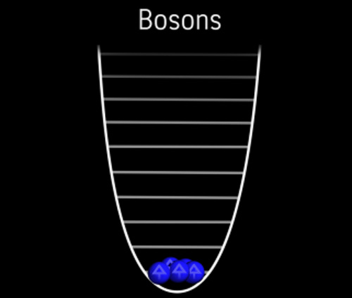
We are now in a position to understand why one would need bosonic atoms to make a BEC: Fermions cannot occupy the same macroscopic quantum state, but bosons can. And, we know how to recognize which atoms will actually be bosons. The first atomic gaseous Bose-Einstein condensates were made in Boulder, Colorado, using rubidium (Rb) atoms; in Cambridge, Massachusetts, using atomic sodium (Na); and in Houston, Texas, using atomic lithium (Li). These three elements are members of the alkali metal family, and share the property of having a single (and thus unpaired) electron outside a fully closed shell of electrons. These unpaired outer shell electrons with their magnetic moments allow them to be caught in a magnetic trap, as seen in Unit 5. If we want gases of these atoms to Bose condense, we must think counterintuitively: We need isotopes with odd values of A, so that the total number of spin-1/2 fermions—protons, electrons, and neutrons—is even. These alkali metals all have an odd number of protons, and a matching odd number of electrons; therefore, we need an even number of neutrons. This all leads to A being an odd number and the alkali atom to being a boson. Thus the isotopes ⁷Li, ²³Na, and ⁸⁷Rb are appropriate candidates, as they are composite bosons.

Figure 21: Atomic de Broglie waves overlap as temperatures are lowered.
Source: © Wolfgang Ketterle.
A particle’s de Broglie wavelength is given by the expression = h/p, where is the wavelength, h is Planck’s constant, and p the momentum. This might make it seem as if the particle’s wavelength were one of its properties like its mass, and its numbers of neutrons, electrons, and protons. However, this is not the case: The value of the momentum (and thus the wavelength) depends on the relation of the motion of the atom to the reference frame of the observer. An observer rushing toward an oncoming atom records a higher momentum and thus a shorter wavelength, as compared to those same quantities as viewed by a second observer rushing away from the approaching particle. This is not a quantum effect but another instance of the familiar Doppler effect, which makes the pitch (actually the frequency) of an approaching ambulance siren seem higher as it approaches, and then lower when passing us by. Thus, in a gas of trapped atoms, the appropriate de Broglie wavelength is that due to the relative momenta of the atoms as they are cooled. Hot atoms are moving quickly relative to one another, and thus have relatively short de Broglie wavelengths, as seen by the other atoms in the gas. As the temperature of the atoms is lowered, the atoms’ relative de Broglie wavelengths lengthen. Once the temperature is low enough that this relative quantum wavelength is long compared to the average distance between the nearest neighbor atoms that Bose-Einstein condensation begins, and a quantum phase transition to a coherent single quantum entity, the BEC, takes place. (Unit: 6)

What does it take to form a gaseous macroscopic quantum system of bosonic atoms? This involves a set of very tricky hurdles to overcome. We want the atoms, trapped in engineered magnetic or optical fields, to be cooled to temperatures where, as we saw in Unit 5, their relative de Broglie wavelengths are large compared with the mean separation between the gaseous atoms themselves. As these de Broglie waves overlap, a single and coherent quantum object is formed. The ultimate wavelength of this (possibly) macroscopic quantum system is, at low enough temperatures, determined by the size of the trap, as that sets the maximum wavelength for both the individual particles and the whole BEC itself.

Einstein had established this condition in his 1924 paper, but it immediately raises a problem. If the atoms get too close, they may well form molecules: Li₂, Rb₂, and Na₂ molecules are all familiar characters in the laboratory. And, at low temperatures (and even room temperatures), Li, Na, and Rb are all soft metals: Cooling them turns them into dense hard metals, not quantum gases. Thus, experiments had to start with a hot gas (many hundreds of degrees K) and cool the gases in such a way that the atoms didn’t simply condense into liquids or solids. This requires keeping the density of the atomic gases very low—about a million times less dense than the density of air at the Earth’s surface and more than a billion times less dense than the solid metallic forms of these elements.

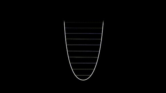
Figure 22: Atoms in a Bose condensate at 0 K.
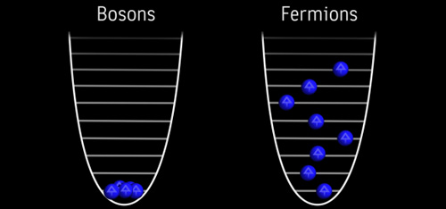
Atoms moving in a harmonic trap occupy quantized energy levels just like electrons in an atom. Bosonic atoms at 0 K are all in the lowest possible motional energy level in the trap; thus, in the highly dilute gaseous BECs, where the particle interactions are very weak, it may be said that all of the atoms are in the same quantum state, which then takes on the properties of a single macroscopic quantum entity. (Unit: 6)

Stating all this in terms of bosonic atoms in quantum energy levels, rather than overlapping de Broglie waves, leads to the picture shown in Figure 22. Here, we see the energy levels corresponding to the quantum motion of the atoms in the magnetic (or optical) trap made in the laboratory for collecting them. As the temperature cools, all of the bosonic atoms end up in the lowest energy level of the trap, just as all the photons in an ideal laser occupy a single quantum state in a trap made of mirrors.

The role of low temperature

The fact that gaseous atoms must be quite far apart to avoid condensing into liquids or solids, and yet closer than their relative de Broglie wavelengths, requires a very large wavelength, indeed. This in turn requires very slow atoms and ultra-cold temperatures. Laser cooling, as discussed in Unit 5, only takes us part of the way, down to about 10^-6 (one one-millionth) of a degree Kelvin. To actually achieve the temperature of 10^-8 K, or colder, needed to form a BEC, atoms undergo a second stage of cooling, ordinary evaporation, just like our bodies use to cool themselves by sweating. When the first condensates were made, no temperature this low had ever been created before, either in the laboratory or in nature. Figure 23 illustrates, using actual data taken as the first such condensate formed, the role of evaporative cooling and the formation of a BEC.

Figure 23: Three stages of cooling, and a quantum phase transition to a BEC.
Source: © Mike Matthews, JILA.
The figure above shows three false color images of the velocity distribution within a cloud of ⁸⁷Rb atoms in a magnetic trap. The fastest atoms are colored red, and as they slow down their colors change to yellow, green, blue, and finally white. Moving from left to right, the three images show successive stages of cooling. The leftmost peak corresponds to an atom cloud at ~10^-6 K. At this temperature, the atoms behave as a classical gas with a relatively broad spread in velocity. Moving toward the right, the subsequent two peaks show the change in the velocity distribution as the trapped atoms are evaporatively cooled (see Unit 5). As the temperature is lowered, the classical gas gives way to a Bose-Einstein condensate with a sharply peaked velocity distribution. In the rightmost image, almost all of the bosonic ⁸⁷Rb atoms are now in the lowest energy level of the trap. The residual non-condensed atoms actually indicate a temperature of ~10^-8 K, a world record low at the time. (Unit: 6)

The process, reported in Science in July 1995, required both laser cooling and evaporative cooling of ⁸⁷Rb to produce a pretty pure condensate. Images revealed a sharp and smoothly defined Bose-Einstein condensate surrounded by many “thermal” atoms as the rubidium gas cooled to about 10^-8 K. By “pretty pure,” we mean that a cloud of uncondensed, and still thermal, atoms is still visible: These atoms are in many different quantum states, whereas those of the central peak of the velocity distribution shown in Figure 23 are in a single quantum state defined by the trap confining the atoms. Subsequent refinements have led to condensates with temperatures just above 10^-12 K—cold, indeed, and with no noticeable cloud of uncondensed atoms. That tells us that all these many thousands to many millions of sodium or rubidium atoms are in a single quantum state.

The behavior of trapped atoms

How do such trapped atoms behave? Do they do anything special? In fact, yes, and quite special. Simulations and experimental observations show that the atoms behave very much like superfluids. An initial shaking of the trap starts the BEC sloshing back and forth, which it continues to do for ever longer-times as colder and colder temperatures are attained. This is just the behavior expected from such a gaseous superfluid, just as would be the case with liquid helium, ⁴He.

The extent of the oscillating behavior depends on the temperature of the BEC. A theoretical computer simulation of such motion in a harmonic trap at absolute zero—a temperature that the laws of physics prevent us from ever reaching—shows that the oscillations would never damp out. But, if we add heat to the simulation, little by little as time passes, the behavior changes. The addition of increasing amounts of the random energy associated with heat causes the individual atoms to act as waves that get more and more out of phase with one another, and we see that the collective and undamped oscillations now begin to dissipate. Experimental observations readily reveal both the back-and-forth oscillations—collective and macroscopic quantum behavior taking place with tens of thousands or millions of atoms in the identical quantum state—and the dissipation caused by increased temperatures.

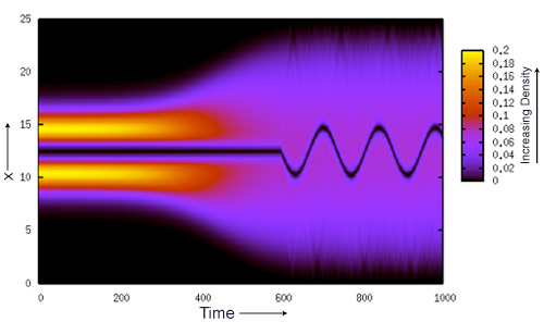
Figure 24: Super-oscillations of a quantum gas and their dissipation on heating.
Source: © William P. Reinhardt.
On the left, we see the oscillations of a pure BEC that has been disturbed somehow. Under ideal conditions, this initially displaced pure BEC will continue to oscillate forever at a temperature of 0 K. The period of these oscillations is determined by the mass of the atoms and the shape of the trap. On the right, we see the effect of slowly adding heat to the condensate over time. As time passes and the temperature increases, the once clear and strongly regular oscillations begin to be quenched, and atoms are lost from the central and still quantum-like core. The main mechanism causing such behavior is decoherence of the overall quantum phase of the condensate. (Unit: 6)

This loss of phase coherence leads to the dissipation that is part of the origins of our familiar classical world, where material objects seem to be in one place at a time, not spread out like waves, and certainly don’t show interference effects. At high temperatures, quantum effects involving many particles “de-phase” or “de-cohere,” and their macroscopic quantum properties simply vanish. Thus, baseballs don’t diffract around a bat, much to the disappointment of the pitcher and delight of the batter. This also explains why a macroscopic strand of DNA is a de-cohered, and thus classical, macroscopic molecule, although made of fully quantum atoms.

Gaseous atomic BECs are thus large and fully coherent quantum objects, whereby coherent we imply that many millions of atoms act together as a single quantum system, with all atoms in step, or in phase, with one another. This coherence of phase is responsible for the uniformly spaced parallel interference patterns that we will meet in the next section, similar to the coherence seen in the interference of laser light shown in the introduction to this unit. The difference between these gaseous macroscopic quantum systems and liquid helium superfluids is that the quantum origins of the superfluidity of liquid helium are hidden within the condensed matter structure of the liquid helium itself. So, while experiments like the superfluid sloshing are easily available, interference patterns are not, owing to the “hardcore” interactions of the helium atoms at the high density of the liquid.

We have mentioned several times that laser light and the bosonic atoms in a gaseous BEC are coherent: The quantum phase of each particle is locked in phase with that of every other particle. As this phase coherence is lost, the condensate is lost, too. What is this quantum phase? Here, we must expand on our earlier discussion of standing waves and quantum wavefunctions. We will discuss what is actually waving in a quantum wave as opposed to a classical one, and acknowledge where this waving shows up in predictions made by quantum mechanics and in actual experimental data. Unlike poetry or pure mathematics, physics is always grounded when faced with experimental fact.

Like vibrating cello strings or ripples in the ocean, quantum wavefunctions are waves in both space and time. We learned in Unit 5 that quantum mechanics is a theory of probabilities. The full story is that quantum wavefunctions describe complex waves. These waves are sometimes also called “probability amplitudes,” to make clear that it is not the wavefunction itself which is the probability. Mathematically, they are akin to the sines and cosines of high school trigonometry, but with the addition of i, the square root of -1, to the sine part. So, the wave has both a real part and an imaginary part. This is represented mathematically as (see sidebar), where the iφ is called the “complex phase” of the wavefunction.

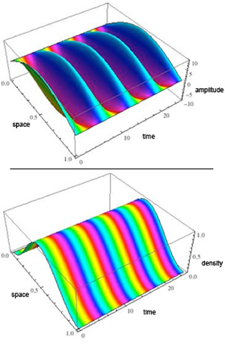
Figure 25: While the complex part of a quantum wavefunction “waves,” the probability density does not.
Source: © William P. Reinhardt.
The mathematical description of a particle makes use of complex numbers, and can be divided into real and imaginary parts. Experiments can only observe the particle’s probability density, which is the absolute value of the wavefunction squared and therefore a real, positive number. However, we can calculate the effects of the complex wavefunction itself. The top image illustrates the ground state wavefunction of a particle trapped in a box. The color scale represents the complex phase of the quantum wavefunction, which is changing periodically in time, and the amplitude of the wave represents the real part of the particle’s wavefunction. If we follow the particle’s time evolution by drawing a line across the graph parallel to the time axis, we see that this quantum amplitude undulates up and down, behaving like a wave. Note that the undulations correspond to the changes in phase. The lower image shows the probability density for the same particle—which would actually be observed in an experiment. We know that the particle is in a stationary state because the density is the same at all times. However, the stripes that correspond to the complex phase of the wavefunction indicate that the underlying complex wavefunction—which we cannot directly observe—is still waving away. (Unit: 6)

The probability density (or probability distribution), which tells us how likely we are to detect the particle in any location in space, is the absolute value squared of the complex probability amplitude, and as probabilities should be, they are real and positive. What is this odd-sounding phrase “absolute value squared”? A particle’s probability density, proportional to the absolute value of the wavefunction squared, is something we can observe in experiments, and is always measured to be a positive real number. Our detectors cannot detect imaginary things. One of the cardinal rules of quantum mechanics is that although it can make predictions that seem strange, its mathematical description of physics must match what we observe, and the absolute value squared of a complex number is always positive and real.  See The Math below.

What about the stationary states such as the atomic energy levels discussed both in this unit and in Unit 5? If a quantum system is in a stationary state, nothing happens, as time passes, to the observed probability density: That’s, of course, why it’s called a stationary state. It might seem that nothing is waving at all, but we now know that what is waving is the complex phase.

For a stationary state, there is nothing left of the underlying complex waving after taking the absolute value squared of the wavefunction. But if two waves meet and are displaced from one another, the phases don’t match. The result is quantum interference, as we have already seen for light waves, and will soon see for coherent matter waves. Experimentalists have learned to control the imaginary quantum phase of the wavefunction, which then determines the properties of the quantum probability densities. Phase control generates real time-dependent quantum phenomena that are characteristic of both BECs and superconductors, which we will explore below.

Phase imprinting and vortices

When does this hidden phase that we don’t see in the experimentally measurable probability density become manifest? The simplest example is in interference patterns such as those shown in Figure 26. Here, the phase difference between two macroscopic quantum BECs determines the locations of the regions of positive and negative interference. So, situations do exist in which this mysterious phase becomes actual and measurable: when interference patterns are generated.

Figure 26: Interference of two coherent BECs, separated and allowed to recombine.
Source: © William P. Reinhardt (left image) and Wolfgang Ketterle (right image).
A BEC may be split into two spatially distinct parts without destroying the phase coherence of the overall macroscopic quantum system. This is accomplished by raising a barrier in the middle of the trap holding the BEC. Once the BEC is so separated, the trap is turned off, and all of the BEC expands. When the expanded separated parts overlap, they show constructive and destructive interference depending on whether the overlapping BECs are in, or out, of phase. The image on the left shows a calculation of the interference pattern, with the x-y plane representing position and the z-axis representing the density of atoms. The right-hand image shows a similar interference pattern in an MIT experiment. The darker areas correspond to areas with a higher density of atoms. In the experiment, two unacquainted condensates (with no prior phase coherence) were allowed to expand and overlap. Interference is still the outcome. (Unit: 6)

But, there is more if we fiddle with the overall phase of a whole superfluid or superconductor with its many-particle macroscopic wavefunction. Imprinting a phase on such a system can create moving dynamical structures called vortices and solitons. Both signify the existence of a fully coherent, macroscopic many-particle quantum system.

A phase can be “imprinted” by rotating such a macroscopic quantum system. This creates vortices as we see in the density profile calculated in Figure 27. Physicists have observed such vortices in liquid superfluids, gaseous BECs, and superconductors. All have the same origin.

Figure 27: Quantum vortices in a BEC (top) and the corresponding phase of the quantum wavefunction (bottom).
Source: © William P. Reinhardt.
A feature common to all macroscopic quantum systems is the formation of vortices. These are quantum whirlpools (or tornadoes) created by rotation, or by phase imprinting via manipulation of atoms caught in a trap. The top image shows the density profile of a BEC with five vortex holes viewed from above. The lower image shows the phase of the same macroscopic wave function leading to the density shown in the upper image, labeled by colors as in Unit 6, Figure 23. Note that the holes in the density occur at exactly those points where the phase is “singular,” that is at those five special points where the diverging colored lines of phase come together. At this point there is no way to assign a phase (a mathematical impossibility.) However, the density is zero at these points, so a choice of phase is meaningless. (Unit: 6)

We can obtain a physical picture of what’s happening if we examine the phase of the underlying macroscopic wavefunction. That’s difficult to do experimentally, but easy if we use a computer calculation to generate the coherent many-body macroscopic wavefunction, as Figure 27 illustrates. Here, unlike in an experimental situation, we fully know the phase of the wavefunction because we have programmed it ourselves. We can then calculate its absolute value squared if we like, which gives the resulting probability density that an experiment would observe. If we calculate the phase in a model of a circulating BEC, superfluid, or superconducting current, and compare it to the observable probability density, we find the phase changes periodically as you trace a circle around what appear to be holes in the probability density, as you can see in Figure 27. Each hole is a tiny quantum whirlpool, or vortex; the lines of phase radiating outward indicate that the quantum fluid is circulating around these holes.

Solitons: waves that do not decay

Figure 28: Density notch soliton.
Source: © William P. Reinhardt.
A type of soliton called a “density notch soliton” can be created in a BEC by manipulating its quantum phase. The image above shows a calculation of a density notch soliton forming in a BEC, with atom density represented by color. The condensate grows until time t = 600 in a trap that splits it into two seemingly distinct (but still coherent) parts separated by a node, as indicated by the black zero-density line down the middle of the image. At t = 600, a laser impinging only on the lower half of the condensate creates a shift in phase between the two halves. The phase shift causes the position of the original node to oscillate: This is the soliton. (Unit: 6)

The vortices and solitons are both highly unusual persistent defects in the quantum wavefunction. Were these systems not macroscopic superfluids, such defects would just disappear and dissipate of their own accord. Try to make a hole in a tub of water and watch it fill in. (On the other hand, lumps of water can propagate without dispersion: Think of tsunamis, where, in exactly the right circumstances, lumps of water can move across a whole ocean.) The same would happen to a quantum bump or dip in the density corresponding to one or a few quantum particles in free space: The wavefunction would spontaneously disperse. It is the collective and coherent nature of the many-particle BEC that allows these nonlinear wave structures to persist. Of course, if you can create a whirlpool as the bathtub drains, it will persist; but such a classical whirlpool has nothing to do with the phase of the liquid water, phase being a purely quantum concept as we apply it here.

Figure 29: The formation of vortices in this BEC shows that it is a superfluid.
Source: © Martin Zwierlein.
This is a picture of a rotating BEC, stirred by a laser. These sodium atoms were laser-cooled, trapped, and cooled further until they condensed into a BEC. Then the cloud of atoms was stirred with a laser to determine whether it was in a superfluid state. One unmistakable characteristic of superfluids is that quantized vortices form when they rotate too quickly. The bright areas in this image are atoms in the BEC, and the dark areas are vortices, which form in a lattice pattern as the cloud is rotated faster and faster. This picture demonstrates unmistakably that this cloud of atoms is in a superfluid state. (Unit: 6)

The vortices and solitons we describe are all consistent with the idea that all the particles are in a single quantum state. These highly dilute gaseous condensates are essentially 100 percent pure, in the sense that all the particles occupy a single quantum state in the trap—although, to be sure, the quantum state wavefunction distorts as the trap is filled. The simple tools developed here have their limitations. They apply to dilute atomic gases, but cannot deal with a more traditional liquid such as ⁴He in its superfluid state. Owing to the very strong interactions between the helium atoms at the much higher density of the liquid, the condensate is only about 10 percent pure condensate. This does not affect its remarkable properties as a superfluid, but certainly makes its theoretical description more difficult. In fact, it makes the quantitative description of the coherent quantum wavefunction a tremendously exciting exercise in computational physics.

We have discussed the fact that a neutral atom of ⁷Li is a boson. That’s because the neutral atom’s three protons, three electrons, and four neutrons add up to an even number of spin-1/2 fermions, thus giving the atom an integral total spin. ⁷Li is the predominant isotope of lithium that occurs naturally on Earth. However, the isotope ⁶Li accounts for about 7 percent of naturally occurring lithium. This isotope has an odd number of spin-1/2 fermion constituents: three protons, three neutrons, and three electrons, and is thus a fermionic atom. What happens to this fermionic isotope of Li if you trap it and cool it down? Rather than Bose condensing like ⁷Li, it fills in the energy levels in the trap just like electrons fill in the energy levels of an atom. A fermionic gas in which the lowest energy levels are occupied with one particle in each level is called “degenerate.” One can thus envisage making an ultra-cold degenerate Fermi gas from ⁶Li, and researchers in the laboratory have actually done so.

Figure 30: Atoms in a trap at 0 K: bosons form a BEC (left) and fermions form a degenerate Fermi gas (right).
Here, we see the ground states of bosons (left) and fermions (right) in harmonic magnetic traps at 0 Kelvin. On the left, we see, as in Figure 22, that all the bosonic atoms are in the unique lowest quantum energy level of the trap. Note that the spins are all pointing in the same direction as their alignment with the trap’s magnetic field is, in fact, what holds them in the trap. Because these atoms are bosons, with integer spin, this does not violate the Pauli exclusion principle. On the right, in strong contrast, each spin-up composite fermionic atom occupies a single energy level. Unlike the pairs of oppositely oriented electrons in Figures 12 and 13, there simply are no spin-down atoms as these are not held in the trap. The situation illustrated on the right is a fully degenerate Fermi gas; if most but not all of the energy levels were occupied, we would have a “partially” or “highly” degenerate gas. The use of the word “degenerate” here simply means that energy levels are occupied from the bottom up. (Unit: 6)

Cooling Fermi gases in that way is far more difficult than making an atomic gaseous BEC. Once physicists learned to make them, gaseous BECs immediately became commonplace. Part of the advantage of making a BEC is the bosonic amplification—the effect of sucking all the bosons into the same quantum state that we encountered in our earlier discussion of lasers. The word “laser” is actually an acronym for “light amplification through stimulated emission of radiation.” Once a single quantum state begins to fill up with bosons, others, miraculously, want to join them.

This is not at all the case with fermions, as their exclusion principle dictates entirely the opposite behavior. In fact, once a cold and partly degenerate Fermi gas begins to form, many of the energy levels are occupied but a (hopefully) small fraction are not. It then becomes very difficult to further cool the Fermi system. As most levels are already full, only the few empty ones are available to accept another atomic fermion. If these are few and far between, it takes a lot of time and luck to have a Fermi particle lose—through evaporative cooling, say—just the right amount of energy to land in one of the unoccupied energy levels. The other levels are blocked by the exclusion principle. Unsurprisingly called “Pauli blocking,” this is a real impediment to making gaseous macroscopic, fully degenerate cold Fermi gases from fermionic atoms. Experimentalists often co-condense ⁶Li with ⁷Li and allow the ⁷Li BEC to act as a refrigerator to cool the recalcitrant ⁶Li atoms into behaving.

Pairing fermions to make bosons

In the style of earlier parts of this unit, we can represent fermionic ⁶Li as ⁶Li↑, with the ↑ now representing the atom’s outer unpaired electron. Here we can, at last, illustrate the pairing of fermions to give bosons—the analog of the Cooper pairing of electrons in a superconducting metal that Unit 8 will develop fully. Combine two fermions and you get a boson. This is simple numerics: Doubling an odd number produces an even number. So, for our example, the molecule ⁶Li₂ must be a boson whether it exists in the higher energy level ⁶Li↑ ↑⁶Li or the lower energy ⁶Li↓ ↑⁶Li. Now you can see why, in a chapter about macroscopic quantum states, we started off with a discussion of simple molecules. We should note, conversely, that combining two bosons just gives another boson, as the number of spin-1/2 particles is still even.

Figure 31: Interference pattern created by the overlap of two clouds of molecular BECs, each composed of 6Li2 diatomic molecules.
Source: © C. Kohstall & R. Grimm
An atom of 6Li is a fermion, with three electrons, three protons, and three neutrons adding together for a total of nine spin-1/2 particles. It’s possible to make a degenerate Fermi gas of 6Li by cooling the atoms in a trap together with bosonic 7Li. To make a BEC out of the Fermi gas, it’s necessary to make the fermionic atoms pair up and form bosons. Researchers in Innsbruck accomplished this by using a carefully tuned laser to induce individual 6Li atoms to form diatomic molecules of 6Li2. Unlike their fermion parents, these bosonic molecules are in identical macroscopic quantum states, and thus form a BEC. When two such clouds overlap, macroscopic interference patterns (compare to Figure 26) immediately appear showing both that pairing of fermions creates bosons, and that these have condensed into coherent matter-wave clouds. (Unit: 6)

Figure 31 indeed shows that fermionic atoms can pair and become molecular bosons, which can then condense into a molecular BEC. This is evident from the striking similarity of the interference patterns shown in Figures 26 and 31. Two overlapping degenerate Fermi gases would not create such macroscopic interference patterns because those wavefunctions have no intrinsic phase relationships, in contrast to the BEC wavefunctions. Molecular BECs, especially if the molecules are polar and can communicate with one another through long-range forces, are of special interest as being quantum information storage devices, as individual molecules can potentially be addressed via their many internal degrees of freedom.

Macroscopic quantum fluids, or superfluids, can be formed from cold bosons. Many types of composite entities fulfill the basic bosonic requirement of integral spin. So, the gaseous quantum superfluid can consist of bosonic atoms, and quite newly bosonic molecules, all of which contain an even overall number of spin-1/2 fermions, be they electrons, protons, or neutrons. All are uncharged superfluids. In the dilute gaseous superfluid phase, they display fully quantum properties, such as interference on the length scale of around a millimeter, which are visible to the naked eye. So, they are certainly macroscopic. Dense liquid superfluids such as ⁴He, of course, contain many more atoms than gaseous BECs in laboratory traps, and have a myriad of unusual properties. But, they do not directly display their fundamental quantum nature quite so directly, even though it underlies their superfluid behavior.

Figure 32: A fountain of superfluid 4He
Source: © Peter Taborek, Low Temperature Materials Laboratory, University of California, Irvine.

Two fermions can pair to make a boson: This allows fermionic ³He to become a superfluid, albeit at a much lower temperature than its bosonic neighbor ⁴He. The pair interaction between these ³He atoms is far too weak to allow formation of molecules in the liquid, so the pair formed is rather ephemeral, and is best described in analogy to what happens to electrons in a superconductor rather than atoms in ⁴He.

Famously, and unexpectedly, even two electrons can pair in a metallic free-electron “sea” to make a composite boson inside a superconductor. This seems odd at first, as these electrons have like charges and thus repel each other. Thus, their pairing is not at all like making bosonic ⁶Li₂ from fermionic ⁶Li, as those atoms actually attract and form molecules in physical space. The pairing of electrons to make bosonic pairs of electrons, called “Cooper pairs,” is indeed more complex. It does not even take place in the three-dimensional coordinate space in which we live. Rather, the pairing occurs in a more abstract “momentum” space. We leave that description to Unit 8, simply noting that it is yet another example of the pairing concepts that we have introduced here. And, because a bosonic pair of electrons carries two units of negative electrical charge, the Bose condensate of such paired electrons is not only a superfluid, but also a superconductor.

Probability Density

The wavefunctions that describe stationary states of quantum mechanical systems have the mathematical form:

ψ(x)e^-iEt/h

where ψ(x) is a real function, and Et/ is called the complex phase of the wavefunction. Each variable has a physical meaning: x is position, E is the system’s energy, and t is time. Using Euler’s formula (see sidebar), we can rewrite this as:

ψ(x)[cos(Et/h)-i sin(Et /ℏ)]

Thus, the quantum wavefunction has both a real part and an imaginary part. The probability density that we would observe in an experiment, however, is proportional to the absolute value of the wavefunction squared:

|ψ(x)[cos(Et/ℏ)-i sin(Et/ℏ)]|²

Which can be rewritten like this:

|ψ(x)[cos(Et/ℏ)-i sin(Et/ℏ)][cos(Et/ℏ)+i sin(Et/ℏ)]

= ψ(x)²[cos²(Et/ℏ) – sin²(Et/ℏ)]

= ψ(x)²

In the first line, we have used the definition of absolute value squared, in the second line we have multiplied the sines and cosines together, and in the third line we have applied the fact that sin²(x) + cos²(x) = 1.

The experimentally observed probability density, therefore, has no imaginary part. It is real and positive, as expected. However, the imaginary part of the wavefunction can make a huge difference in how two quantum mechanical objects interact, as we have seen in the quantum interference of particles in Unit 5 and will see in the quantum interference of BECs in this unit.

• Eric A. Cornell and Carl E. Weimann, “The Bose-Einstein Condensate” Scientific American, March 1998.
• Eric A. Cornell, Carl E. Weimann, Wolfgang Ketterle: Nobel Prize Lectures, available at http://nobelprize.org/nobel_prizes/physics/laureates/2001/index.html.
• Wolfgang Ketterle, “How are temperatures close to absolute zero achieved and measured?” Scientific American.com, Ask the Experts, January 19, 2004, found here: http://www.scientificamerican.com/article.cfm?id=how-are-temperatures-clos.
• Carlos A.R. Sa de Melo, “When fermions become bosons: Pairing in ultracold gases” Physics Today, Oct. 2008, p. 45–51.
• Eric R. Scerri, “The Periodic Table, Its Story and Significance” Oxford University Press, 2007.
• Charles Townes, “How the Laser Happened: Adventures of a Scientist” Oxford University Press, 2002.